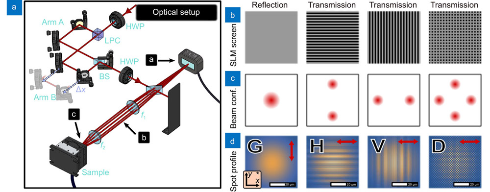
Fig. 1. (a) Experimental setup. Abbreviations: half-wave plate (HWP), linear polarizing cube (LPC), beam splitter (BS), spatial light modulator (SLM), focusing lenses (f₁,f₂). (b) SLM function. (c) Spot profile distribution at the sample: Gaussian (G) and DLIP (V, H, D) profiles. (d) The red arrow indicates the polarisation vector.

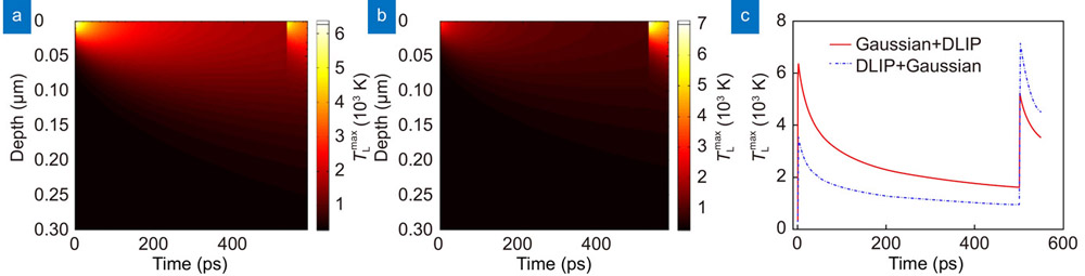
Fig. 2. TLmax evolution at different depths for (a) G₁= 1, G₂= 0 and (b) G₁= 0, P₂=1, after irradiating a flat profile (NP= 1) with E= 25 μJ, Δτ = 500 ps. (c)TLmax on the sample surface as a function of time in the cases shown in (a) and (b).

Fig. 3. (a) Spot intensity distribution. (b) SEM images of processed surface. (c) Fourier transform diagrams, produced by trains of single pulses. The total number of pulses is NP = 50, the energy per pulse is E_tot = 80 μJ for G, and E_tot = 57 μJ for the DLIP distribution V, H and D. The red arrow in A indicates the polarisation direction.

Fig. 4. SEM images of the double pulse irradiation schemes used (1^st column) together with the respective FFT analyses (2^nd column) and simulation results (columns 3−5).The pulse profile and the order are indicated in the legends of the 1^st column, while the superscript arrows indicate the pulse polarization in each case. The total energy of the double pulse pair is 80 μJ/pulse and NP = 50 pulses. Simulation results are shown in each case, just before (3^rd column, Δ τ = 490 ps) and right after (4^th column, Δ τ = 520 ps) the arrival of the second pulse. The final morphology predicted by the simulation experiment is shown in the 5^th column (contour plots to illustrate the height). The arrows in the 3^rd and 4^th column provide a guide to eye representation of the fluid transport direction. The color bars at the bottom of the figure provide the temperature (3^rd and 4^th columns) and height (5^th column) values range.

Fig. 5. Stainless steel surface morphology following variation in pulse energy and NP, as indicated in the respective legends, for the D+ G pulse sequence case. The corresponding result of theoretical simulations for 20 μJ pulse energy is shown as an inset defined by the dashed rectangle, illustrating (i) the temperature profile for NP = 50 and t = 520 ps and (ii) the final surface morphology for NP = 50.

Fig. 6. Complex structures generated with E_tot = 70 μJ, NP = 100 with the D+G pulse sequence irradiation scheme. The SEM image is analysed with FFT and reconstructed surfaces comprising structures at different length scales are illustrated. The areas corresponding to the different periodicities are highlighted in FFT diagrams.

Fig. 7. Simulation results showing the surface temperature profile obtained for the G+V case at different time moments and NP, as indicated. The arrows in the figures in the zoomed regions illustrate the spatial distribution of the magnitude and direction of the calculated fluid velocity vectors.