
Wensong Wei, Yankun Peng, Xiaochun Zheng, Wenxiu Wang, Fang Tian. Rapid Determination of Content of Total Volatile Basic Nitrogen in Pork Based on Multispectral Detection System with Optimal Wavelength[J]. Acta Optica Sinica, 2017, 37(11): 1130003
- Acta Optica Sinica
- Vol. 37, Issue 11, 1130003 (2017)
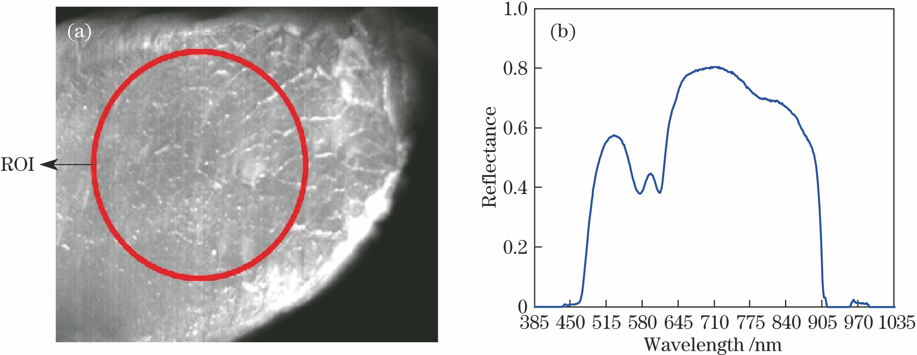
Fig. 1. (a) Hyperspectral image at wavelength of 280 nm of ROI and (b) reflectance curve after calibration of a certain sample

Fig. 2. Raw reflectance spectra of 52 pork samples
Fig. 3. Spectrograms of raw spectra after preprocessing with FD-SNV algorithm
Fig. 4. (a) Number of characteristic wavelength screened by SWA algorithm; (b) wavelength distribution of screening variable
Fig. 5. Regression coefficient distribution of band screened by SWA algorithm
Fig. 6. (a) Number of optimal characteristic wavelength screened by SPA algorithm; (b) detailed position of characteristic wavelength
Fig. 7. (a) Frequency of characteristic wavelength screened by GA algorithm; (b) modeling contribution rate of characteristic wavelength number
Fig. 8. Distribution of characteristic wavelength screened by GA algorithm
Fig. 9. Distribution of optimal characteristic wavelength screened by three algorithms of SWA, SPA, and GA
Fig. 10. Diagram of multispectral detection system
Fig. 11. Reflectance of 44 pork samples collected by multispectral method
Fig. 12. Predicted content of TVB-N with PLSR model and MLR model. (a) PLSR model, calibration set; (b) PLSR model, prediction set; (c) MLR model, calibration set; (d) MLR model, prediction set
|
Table 1. Measured mass fraction of TVB-N in calibration set and prediction set of the first group pork samples
|
Table 2. Measured mass fraction of TVB-N in calibration set and prediction set of the second group pork samples
|
Table 3. PLSR model results of raw spectra after preprocessing with different methods
|
Table 4. Modeling results of characteristic wavelength obtained by different screening variable algorithms
|
Table 5. Predicted results of PLSR model and MLR model established by multispectral method

Set citation alerts for the article
Please enter your email address
© Copyright 2018-2021 | Chinese Laser Press. All Rights Reserved 沪ICP备15018463号-20