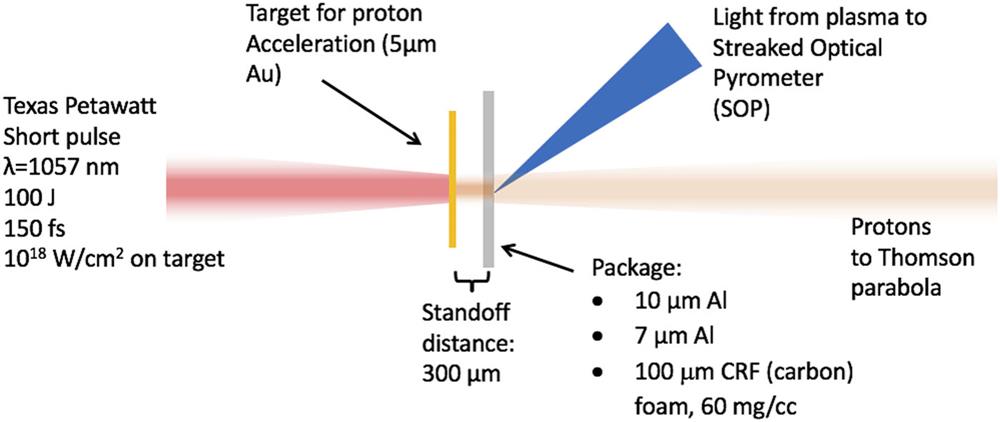
Fig. 1. Schematic of experiment. The short-pulse Texas Petawatt Laser (TPWL) accelerates protons off the first target, and the proton beam deposits energy and heats the second target (package). The second target emits blackbody radiation that is measured by the streaked optical pyrometer (SOP), while the energies of the protons that are not stopped in the package are measured by the Thomson parabola spectrometer (TPS). Adapted with permission from Roycroft et al., AIP Adv. 10, 045220 (2020). Copyright 2020 AIP Publishing LLC.

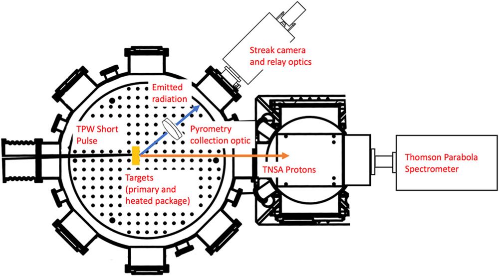
Fig. 2. Layout of experiment inside TPWL vacuum chamber. The target normal sheath acceleration (TNSA) protons that pass through the target are diagnosed by the TPS, while blackbody radiation from the target is captured and imaged onto the slit of the SOP.

Fig. 3. Microscope image of a mounted target. The gold foil is glued to the far side of the stalk. A heating package would be glued to the near side to create the necessary 300-µm spacing. To allow accurate imaging of the diagnostics on either side of the stalk, small wires are glued to the sides of the stalk.

Fig. 4. (a) Expected brightness temperature as a function of streak-camera counts, calculated from blackbody formula and calibration for optics transmission and streak-camera settings. The streak camera saturates at 4095 counts, and we attempt to run the experiment at a setting where the maximum brightness temperature occurs near but below the saturation point. The dashed red lines are the upper and lower bounds for the brightness temperature based on the measurement uncertainties. (b) Streak-camera image converted from counts to brightness temperature (shot 11 441; package: 10-μm aluminum). Adapted with permission from Roycroft et al., AIP Adv. 10, 045220 (2020). Copyright 2020 AIP Publishing LLC.

Fig. 5. (a) Assumed spectrum, (b) dE/dX, and (c) fraction of spectrum stopped in each zone for sample proton spectra, all for shot 11 477. The package is 100-μm-thick CRF and the zone size is 1 µm.

Fig. 6. (a) Density profiles at 0 ps, 100 ps, and 500 ps for a sample aluminum-foil simulation (shot 9626). (b) Temperature profiles at 0 ps, 100 ps, and 500 ps for the same simulation as in (a), along with vertical lines showing the location of the 400-nm critical density at 100 ps and 500 ps.

Fig. 7. (a) Density profiles at 0 ps, 100 ps, and 500 ps for a sample CRF simulation (shot 11 477). (b) Temperature profiles at 0 ps, 100 ps, and 500 ps for the same simulation as in (a).

Fig. 8. (a) Material temperature and resulting optical depth for sample CRF simulation (shot 11 477) at 0 ps. (b) Material temperature and resulting optical depth for the same simulation at 500 ps.

Fig. 9. Post-processing of simulation of 10-μm aluminum-foil package (shot 9626) using both opacity–photosphere processing and n-critical processing. The processes give identical equivalent temperatures early on, but the opacity processing delivers lower equivalent temperatures later in the simulation. Regarding the background in the SOP images, below the simulation t = 0, there was background light from the laser flash, and at t ≈ 400 ps there was reflection from the optics in the chamber, creating a spike in the SOP reading at that point.

Fig. 10. (a) SOP lineout and three xRAGE simulations for shot 11 477, which was hotter and had less noise on the SOP than shot 11 485, shown in (b). The calculations are shown with an energy ramp and without (simply adding all of the energy at the starting point). The laser-to-ion-beam energy conversion efficiency is shown for both the cutoff and exponential-fit spectra.

Fig. 11. Models of warm and hot DQ atmosphere temperature and density, plotted alongside the same parameters in the xRAGE CRF simulations. The hot DQ models have a pure carbon composition, while the warm DQ models have N(C)/N(He) = 0.1. The electron density in the experiment is three to four orders of magnitude higher than the electron density for the DQ white-dwarf atmospheres.

Table 1. Laser energy to TNSA proton energy for each sample shot discussed herein; the energy conversion is based on the value of N_ions needed to heat the package to the measured temperature on shot.