We are motivated to study warm dense matter (WDM) because of its prevalence in many physical systems relevant to high-energy-density physics, including imploding inertial-confinement-fusion capsules and astrophysical bodies such as stellar and giant-planet interiors. WDM is defined as a state of matter in which the Coulomb coupling parameter and the electron degeneracy parameter are both of order unity, thereby making it difficult to calculate the equation of state (EOS) and other transport properties. In the present experiment on heated carbon foam, the coupling parameter was near unity and the degeneracy parameter (the ratio of the kinetic energy to the Fermi energy) was between 2 and 8 depending on the shot. The present exploratory work was to determine whether we could (i) create and diagnose warm dense carbon plasmas with our isochoric heating platform and (ii) understand the results of our diagnostics via radiation-hydrodynamics modeling.

The motivation for the present work was to achieve laboratory conditions that are analogous to those in the atmospheres and envelopes of white-dwarf stars with carbon lines [DQ white dwarfs (DQWDs)] by heating carbon foams to between ∼1 eV and 2 eV. However, the present work is also broadly applicable to studying the WDM EOS, which in many cases is not well constrained. White dwarfs are of interest as the final evolutionary phase for around 97% of all stars in the universe, most of which have either hydrogen- or helium-rich atmospheres. DQWDs constitute a class of helium-rich white dwarfs with substantial concentrations of carbon in their atmospheres, which is relevant to our carbon-foam experiments. The atmospheres of the subclass of hot DQWDs have effective temperatures in the range of 18 000–25 000 K (1.5 eV–2 eV).^1–3 DQWD atmospheres have electron densities of up to 10¹⁸ cm⁻³, while their envelopes have electron densities of up to 10²³ cm⁻³. This density–temperature regime is within the WDM parameter space, therefore laboratory studies can provide benchmarks for theoretical models of white-dwarf atmospheres and envelopes.^4,5 However, note that measuring the carbon EOS or spectral lines will require diagnostics beyond those used in the present experiment. Kritcher et al.⁵ emphasized recently the current interest in white-dwarf EOS properties, although they examined the behavior of the principal Hugoniot at pressures and temperatures far higher than those that we achieve with isochoric heating.

We can create WDM at the Texas Petawatt Laser (TPWL) facility by means of our isochoric heating platform, where we heat samples with a laser-accelerated proton beam on approximately picosecond timescales and probe them as they expand on approximately nanosecond timescales. Short-pulse lasers are ideal for isochoric heating experiments because of the amount of energy they can deliver on an approximately picosecond timescale; it is possible to heat matter with laser-accelerated proton beams,⁶ laser-accelerated ion beams,^7,8 and even direct heating from the laser pulse.⁹ For our isochoric heating platform, we use protons with approximately megaelectronvolt energy and accelerated via the target normal sheath acceleration (TNSA) mechanism^10–12 that arises from the short-pulse laser interaction with 5-μm-thick gold targets. Having heated the foam or foil to WDM conditions, we measure the surface brightness temperature with a streaked optical pyrometer (SOP).¹³ We can also measure the transmitted proton spectrum for energies above ∼1.5 MeV on each shot with a Thomson parabola spectrometer (TPS).

To interpret the pyrometry data, we perform radiation-hydrodynamics simulations of the heated material. Because our eventual goal is to use our experimental measurements in conjunction with modeling to evaluate performance of different EOS tables and other models for this regime, it is important to have a modeling platform in place, including proper post-processing. This is consistent with other recent WDM experimental studies, which included complementary radiation-hydrodynamics simulations.^14,15 For the simulations, we use the proton energy spectrum from a TPS to set up the initial simulation conditions. We use cold stopping powers from the Stopping and Range of Ions in Matter (SRIM) database to calculate the proton dE/dx, which becomes a spatial internal energy (SIE) profile that we then use as the energy source for our xRAGE simulations, in a manner described by Bang et al.⁷ This dE/dx calculation is necessary because xRAGE contains no physics regarding ion energy deposition. The simulated material then expands into a low-density background gas, and the material temperature in the simulated material is compared to the SOP measurements. We found that while optically thick materials (e.g., aluminum) conform to the idea of having an “emitting layer” (first discussed in 1993 by Celliers and Ng¹⁶) around the critical surface of the wavelength viewed by the pyrometer, we needed to post-process the foam simulations differently to account for the partial transparency of the foam.

In this paper, we present our experimental methods in Sec. II, simulation methods in Sec. III, and results from probing and analyzing warm dense aluminum and carbon foams in Sec. IV, with an eye toward eventual applications in comparison with EOS theory. We demonstrate that we can create and observe the brightness temperature of warm dense carbon foams with a density of 60 mg/cm³. In Sec. III, we present our post-processing technique for comparing our xRAGE radiation-hydrodynamics simulations with the brightness temperature measurements of the carbon foams. In Sec. V, we discuss applications of the experiments for eventual EOS measurements, and the relevance to DQWD atmospheres and envelopes.

The experiments were performed at the TPWL facility,^17,18 which delivers a short-pulse beam with 150-fs pulse duration and up to 150 J of energy. Its intensity contrast was measured in 2017 (see supplementary material) to be ∼5 × 10⁸ at 50 ps. It is amplified by optical parametric chirped pulse amplification followed by pulsed power amplification delivered by means of flashlamps in neodymium-doped glass. The short-pulse beam can be focused either by an f/3 off-axis parabola into the TC1 target chamber or by an f/40 spherical mirror into the TC2 target chamber.

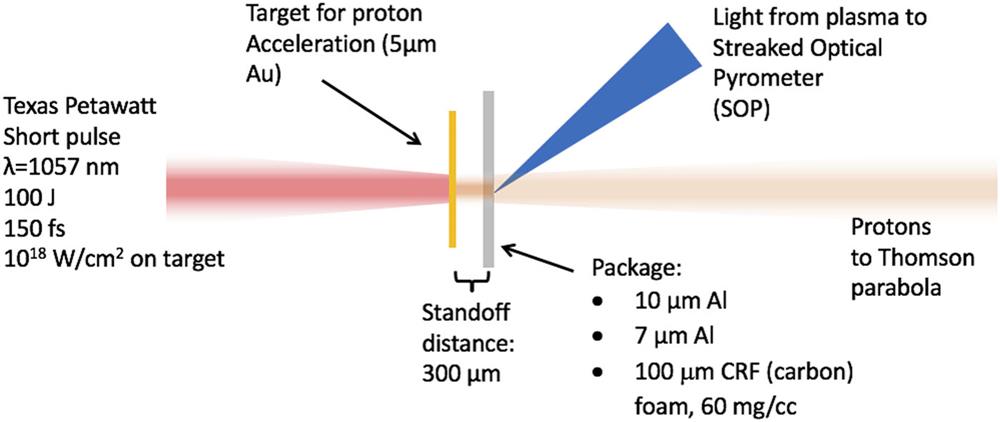
The short-pulse TPWL beam is focused by an f/40 spherical mirror and irradiates a solid gold target with a spot size of around 100 µm. This laser–target interaction produces protons with energies of up to ∼10 MeV and accelerated by TNSA. A secondary target (called the package) is mounted 300 µm behind the ion source and is heated by the proton beam to WDM conditions. Figure 1 shows the experiment schematically.

The target is positioned nearly normal to the laser beam, and the package is mounted directly behind and parallel to the target. Given the nature of standard TNSA interactions, we assume that the majority of the laser–target interaction occurs at the front of the target and that much of the laser light is reflected; the target is therefore angled at around 2° to prevent reflections back up the laser chain. The SOP images the rear surface of the package, while the TPS is placed behind the target to measure the energies of the TNSA protons. Figure 2 shows the layout of the experiment in the target chamber.

The TNSA targets were 5-μm-thick gold foils, while the heating packages were 7-μm and 10-μm-thick aluminum foils or 100-μm-thick 60-mg/cc CRF (carbon) foams.¹⁹ Here, CRF stands for carbonized resorcinol-formaldehyde; the primary component is carbon, and we treat it as purely carbon in our simulations. We have measured the pore size in the foams to be less than 1 µm. We chose aluminum foils for our experiments because aluminum is a standard choice for WDM experiments and has been studied extensively.^6,9,20 There is a modern EOS for aluminum in the SESAME database.²¹ Once we were able to observe heating in aluminum with our diagnostics, we moved on to the experimental package, namely the 60-mg/cc CRF foam.

The targets were mounted on either side of 300-μm-thick aluminum stalks, each with a 2-mm-diameter hole. The stalk provided the spacing between the proton source and the heated package. Figure 3 shows a microscope image of a mounted target (with no heating package). We position the target such that the short-pulse beam hits the middle of the hole, but having a 2-mm target size mitigates the uncertainty in laser pointing and shot-to-shot jitter.

The two diagnostics for this experiment were the TPS,^22,23 which was used to measure the energy spectrum of the protons accelerated via TNSA, and the SOP, which was used to measure the time-resolved blackbody emissions of the heated package.

Optical pyrometry is a standard diagnostic for determining plasma temperature from emission of optical radiation.^24–28 The SOP used in this experiment was designed, built, and calibrated at the University of Texas.¹³ It is an optical telescope that collects the blackbody radiation from the heated package through a bandpass filter centered at 400 nm. A streak camera sweeps the received signal, resulting in an image with one dimension in distance and one dimension in time. Using calibration of the optics and streak-camera response, the radiation is then converted into a brightness temperature in electronvolts. Figure 4 shows SOP sample data; Fig. 4(a) shows an example of a conversion from counts to brightness temperature, and Fig. 4(b) shows a resulting streak-camera image of temperature as a function of distance and time.

Figure 4(b) shows a sample streak-camera image where camera counts have been converted to brightness temperature though the calibration data in Fig. 4(a). The SOP measures both the spatial extent of the heating (in one dimension) and the time evolution of the heating. The resolution for this image is around 5 ps in time and 0.26 ± 0.02 pixels/μm in distance. Both the time resolution and the distance resolution can change based on the SOP settings; these settings are discussed in depth in Ref. 13. For the experiments discussed here, our primary interest is in the time evolution of the heating. However, for other applications such as heating a target with different material components by the same ion beam,⁸ the measurement of heating as a function of distance across the target is also needed. The measurement of the spatial extent of the heating is also an indirect measurement of the proton-beam divergence as it crosses the 300-μm vacuum gap between the TNSA source and the target, as well as its divergence within the target (because this measurement shows only the blackbody radiation from the back surface of the target). For the experiments discussed herein, the spatial extent of the heating varied from shot to shot but was consistently in the range of 300 µm–500 µm.

The experiments are simulated in one dimension using xRAGE,²⁹ an Eulerian radiation-hydrodynamics code developed at Los Alamos National Laboratory (LANL). As an Eulerian code, the fluid moves through a fixed grid, with adaptive mesh refinement to resolve regions of interest in more detail. The relevant physics models used in these simulations are hydrodynamics and partial ionization. We considered 3T physics, thermal conduction, and radiation diffusion (using a multigroup diffusion model), but tests showed those were all small effects in this temperature–density regime.

To justify further why 3T physics produces only a small effect in this simulation work, our simulations showed an electron–ion temperature equilibration time of less than 50 ps if all energy has been deposited into the ions initially. Furthermore, this equilibration has no effect on the final post-processed simulation result. We use the default electron–ion coupling supplied by xRAGE [given by Eq. (3.61) in Ref. 30]; however, we acknowledge that there has been some work showing that the electron–ion equilibration may be slower in the WDM regime than most models predict,³¹ so 3T physics may have some unaccounted-for effect in this regime.

The experiment is modeled by setting a starting density and temperature for each region of the material, and then allowing the material to cool and expand into a low-density background gas. We model the CRF foam as a uniform sample of carbon with a starting density of 0.06 g/cm³, which means an implied porosity of around 97%. We check to see what affect this porosity might have on the foam behavior. We measure the maximum pore size of the foam to be less than 1 µm, and many pores are smaller. We use the estimate of the sound speed in the heated plasma as cs=ZkBTemi1/2. The ion density corresponding to the foam density of 60 mg/cm³ is 2.88 × 10²¹ atoms/cm³ and the free-electron density is given by our xRAGE simulations (∼1 × 10²¹ electrons/cm³), so we have Z ≈ 0.3. This gives c_s = 1.6 µm/ns for T_e ≈ 1 eV and c_s = 2.7 µm/ns for T_e ≈ 3 eV. Therefore, the pores close on time scales of at most a few hundred picoseconds, which is far slower than the isochoric heating. This means that the foam lattice is heated uniformly and then expands inwardly uniformly to close the pores, as well as expanding outwardly. After 100 ps–500 ps, the foam lattice has transformed into a uniform expanding plasma. Our SOP diagnostic resolution cannot resolve the pores, so it sees only a uniformly heated plasma.

The resultant SIE is sourced into xRAGE, which has no model for proton energy deposition physics. The free parameter N_ions is selected to give the starting temperature that matches best with the SOP observations. Note that N_ions is not the only possible free parameter in this simulation: we also ramp the proton energy deposition over time to simulate the rise in proton heating in accordance with the proton time of flight (∼30 ps to cross the 250-μm vacuum gap, plus the time to arrive at the back surface of the given target). In the following paragraphs, we show the step-by-step implementation of the calculation described by Eq. (1).

First, we calculate the stopping power (dE/dX) for each zone of the material. We acknowledge that there is an effort to develop warm stopping power models,³³ although we have used cold stopping power data to set up these simulations. Furthermore, for this experiment, the TPS did not measure counts for protons with energy less than ∼1 MeV. Therefore, we made both a lower-bound estimate for the low-energy proton trend (i.e., a flat count for number of ions below the cutoff) as well as an upper-bound estimate, by fitting the spectrum to a simple exponential (y = ae^−bx), as in Ref. 34. The three proton spectra (no low-energy protons, cutoff assumption for low-energy protons, and exponential fit for low-energy protons) are shown in Fig. 5(a). The energy deposited per proton into each zone of the material (in this case, CRF foam at 60 mg/cm³) for the spectra in Fig. 5(a) is shown in Fig. 5(b). The fraction of the proton spectrum (with low-energy protons) shown in Fig. 5(a) that is stopped in each zone of the material is shown in Fig. 5(c).

The proton spectrum with the highest number of low-energy protons (i.e., the exponential fit) couples energy more effectively from the beam into the heated package. However, for the two dE/dX profiles ^{[Fig. 5(b)]}, the relative amount of energy deposited at each point in the package is the same. We note that even for the exponential-fit spectrum, only a very small fraction of the protons are stopped in the sample, as shown in Fig. 5(c). The low-energy protons are indeed responsible for the majority of the heating, so they must be included in the setup for the simulation. However, because the two dE/dX profiles differ only in magnitude, using one spectrum or the other to initialize the simulation turns out to affect only the free parameter N_ions and therefore the laser-energy to proton-energy conversion factor, which is discussed further below and reported in Table I.

In this experiment, the TPS diagnostic was not calibrated for number of ions; therefore, a range of reasonable values is chosen for N_ions, consistent with ∼1% laser-energy to proton-energy conversion. For each sample shot discussed herein, Table I gives the laser-energy to proton-energy conversion needed to heat the package to the observed temperature. The literature-quoted value for highest laser-energy to proton-energy using TNSA is 9%.³⁵ While the values in Table I are lower, this is expected because we were using a less tightly focused short-pulse beam; laser-to-proton energy conversion is expected to depend on the laser intensity on the target.³⁶

After the initial energy input, the material cools and expands into the vacuum, which we model as a low-density background gas (for these simulations, deuterium at 1 × 10⁻⁴ g/cm³). We read out profiles of material properties as a function of distance (e.g., density in each zone, material temperature in each zone) at each timestep. Figure 6 shows profiles at 0 ps, 100 ps, and 500 ps of material density and temperature for a simulation of a 10-μm-thick aluminum-foil package (shot 9626).

To compare the SOP lineouts with xRAGE, post-processing of the material temperature profiles is needed (note that when considering radiation diffusion, we found the radiation temperature to be equivalent to the material temperature throughout the simulated package). The literature^13–15 shows that for optically thick heated packages starting at solid density, it is sufficient to compare the material temperature at a given “emitting layer” (i.e., the layer from which most of the thermal emission comes from) and the temperature read by the pyrometer, given that the optical depth [defined as τ = ρ ∗ κ ∗ s (density ∗ opacity ∗ optical path length), a dimensionless parameter] of the aluminum foils at this temperature is around 200. This emitting layer is near the critical density surface for the wavelength observed by the SOP. In Fig. 6(b), we plot the location of the 400-nm critical density on the temperature profiles. We calculate that location for each timestep, using electron density profiles calculated by xRAGE. We then plot a temporal lineout of the SOP image against the critical surface temperature at each time.

By contrast, the CRF foams start out as being underdense compared to n_cr for 400-nm light, so calculating a critical density location is impossible. Figure 7 shows profiles at 0 ps, 100 ps, and 500 ps of material density and temperature for a simulation of shot 11 477 (the package was ∼100-μm-thick CRF with a starting density of 60 mg/cm³). For the simulations shown in Fig. 7, we used SESAME EOS 7834.³⁷ For 400-nm light, the foams have an optical depth of ∼2, so radiation comes from throughout the foam. Therefore, we must perform a photosphere calculation.

For this calculation, we find the specific intensity of the light emitted (from the simulated foam) and convert it into an equivalent blackbody temperature, which can then be compared to the SOP lineout data. This calculation follows the “fundamentals of radiative transfer” discussion by Rybicki and Lightman.³⁸

We evaluate the solution to the radiative transfer equation dI/dτ = −I + S, where I is the specific intensity, S is the source function, and τ is the optical depth. The solution for the transfer equation with a constant source is I(τ) = I(0)e^−τ + S(1 − e^−τ), which means that the light coming from any material is equal to the light from the backlighter I(0) diminished by e^−τ plus the self-emission represented by the source function. This form of the solution is useful for estimating the light intensity from any material, although for our calculation we take into account a non-constant source and changing optical depth.

We use opacity data^39,40 from LANL for all of these calculations. Our first step is to calculate the optical depth τ = ρ ∗ κ ∗ s at each point in the material. The optical depth at two different simulation time steps for a sample CRF shot (shot 11 477) is shown in Fig. 8.

After computing the blackbody function, path length, and optical depth at every point in the material for a given timestep, we evaluate Eq. (2) to obtain the specific intensity at that timestep. The intensity is then converted into an equivalent blackbody temperature and plotted against the SOP lineout at each timestep, allowing for direct comparison between the simulation and pyrometry measurement.

Ideally, both post-processing methods should give similar results for the aluminum-foil shots, where the optical depth is large (τ ≫ 1). Using both methods on a single simulation for the example aluminum-foil shot (shot 9626; see Fig. 9), the resulting equivalent temperatures are nearly identical for the first 100 ps of the simulation, with the opacity processing coming out marginally lower as the simulation progresses. The simulations in Fig. 9 have no energy ramp; instead, the simulation starts with the energy of the entire proton beam at t = 0. We set the simulation t = 0 as a time when the SOP measurement is sufficiently above the background.

Comparing the example aluminum SOP data (see Fig. 9) and the CRF SOP data (see Fig. 10) shows that the foam does not cool in the same way as does the aluminum. Unlike with the aluminum shots, the SOP shows little cooling of the CRF target; the temperature does not drop after the initial slight amount of cooling. However, with our post-processing method that accounts for partial transparency, the simulations account for the (lack of) cooling.

We succeeded in measuring the heating and proton spectra concurrently for two different temperature shots of heated 60-mg/cm³ CRF packages, namely shots 11 477 and 11 485. Figure 10 shows SOP lineouts for brightness temperature as a function of time, plotted against three xRAGE simulations for each shot, showing an upper, middle, and lower bound for laser-energy to proton-energy conversion.

While these two shots were taken under similar conditions, a much higher peak brightness temperature was achieved on shot 11 477 because of more ions being accelerated and better coupling to the TPWL short-pulse beam (notably, the laser energy recorded for shot 11 485 was higher than that for shot 11 477; see Table I). Such variation can be understood from changes in the focus of the laser on the primary target (the 5-μm-thick gold foil that is the source of the TNSA protons).

In this paper, we have presented an experimental and simulation platform for studying the WDM created by isochoric heating of carbon foam packages with a laser-accelerated TNSA proton beam. We showed that post-processed xRAGE simulations do a good job of matching the cooling trend for the first 500 ps of the experiments. We also showed that the opacity–photosphere method of processing the xRAGE simulations is necessary for processing simulations of foam packages. For optically thick aluminum foil targets, this processing method produced nearly the same result as reading the temperature from an “emitting layer” at n-critical.

A potential application of our CRF foam results is to help constrain the properties of carbon-atmosphere (DQ) white dwarfs. We compare our carbon foam plasma conditions with modern DQWD atmospheres^41,42 in Fig. 11. The temperature of our two shots is consistent with DQ atmospheres, but our electron densities are between 10²⁰ cm⁻³ and 10²¹ cm⁻³, which is three to four orders of magnitude higher than the atmosphere densities. These densities would correspond to the envelope, below the atmosphere. This higher-density case would still be of considerable interest for an EOS measurement, given that Bergeron et al.⁴³ showed that pressure ionization has a strong effect on the ionization balance. Note that to probe the pressure ionization regime of white-dwarf envelopes, the foam would have to have a higher density (∼10²³ cm⁻³ or 1 g/cm³) and be considerably hotter (∼50 eV). Temperatures in this range are achievable with isochoric heating platforms and have been observed in experiments that were optimized for high temperature, using methods such as ion beam focusing.⁴⁴ Alternatively, we could have a future experiment start with a carbon vapor at less than 1 mg cm⁻³ to probe conditions closer to DQ atmosphere conditions. Another application of our results would be to explore the effects of partial ionization of mid-Z elements at near-solid densities.

With additional diagnostics, such as a Fourier domain interferometer to measure expansion and plasma reflectivity and/or radiography to measure expansion, as well as an optical spectrometer to measure photospheric spectral lines, this experimental and simulation platform could be used to measure EOS and also to compare with astrophysical theories regarding white-dwarf spectra.

References

[1] G. Fontaine, G. Michaud, C. Pelletier, G. Wegner, F. Wesemael. Carbon pollution in helium-rich white dwarf atmospheres: Time-dependent calculations of the dredge-up process. Astrophys. J., 307, 242(1986).
[2] L. G. Althaus, A. H. Córsico, E. García-Berro, A. D. Romero. Hot C-rich white dwarfs: Testing the DB-DQ transition through pulsations. Astron. Astrophys., 506, 835-843(2009).
[3] S. O. Kepler, D. Koester. Carbon-rich (DQ) white dwarfs in the sloan digital sky survey. Astron. Astrophys., 628, A102(2019).
[4] J. E. Bailey, R. E. Falcon, T. A. Gomez, M. H. Montgomery, T. Nagayama, G. A. Rochau, D. E. Winget. Laboratory measurements of white dwarf photospheric spectral lines: Hβ. Astrophys. J., 806, 214(2015).
[5] B. Bachmann, L. X. Benedict, G. W. Collins, T. Döppner, J. L. DuBois, F. Elsner, G. Fontaine, J. A. Gaffney, A. L. Kritcher, D. C. Swift et al. A measurement of the equation of state of carbon envelopes of white dwarfs. Nature, 584, 51(2020).
[6] M. Allen, T. E. Cowan, M. E. Foord, M. H. Key, A. J. Mackinnon, P. K. Patel, D. F. Price, H. Ruhl, P. T. Springer, R. Stephens. Isochoric heating of solid-density matter with an ultrafast proton beam. Phys. Rev. Lett., 91, 125004(2003).
[7] B. J. Albright, W. Bang, J. C. Boettger, P. A. Bradley, J. C. Fernandez, E. L. Vold. Uniform heating of materials into the warm dense matter regime with laser-driven quasimonoenergetic ion beams. Phys. Rev. E, 92, 063101(2015).
[8] B. J. Albright, W. Bang, D. Cort Gautier, G. Dyer, A. Favalli, J. C. Fernández, C. Huang, J. F. Hunter, J. Mendez, S. Palaniyappan et al. Laser-plasmas in the relativistic-transparency regime: Science and applications. Phys. Plasmas, 24, 056702(2017).
[9] J. Abdallah, U. Andiel, K. Eidmann, P. Hakel, G. C. Junkel-Vives, R. C. Mancini, F. Pisani, K. Witte. X-ray spectroscopy of dense plasmas produced by isochoric heating with ultrashort laser pulses. AIP Conf. Proc., 730, 81(2004).
[10] T. E. Cowan, S. P. Hatchett, E. A. Henry, M. H. Key, T. W. Phillips, M. Roth, T. C. Sangster, M. S. Singh, R. A. Snavely, M. A. Stoyer et al. Intense high-energy proton beams from petawatt-laser irradiation of solids. Phys. Rev. Lett., 85, 2945(2000).
[11] T. E. Cowan, S. Hatchett, M. H. Key, A. B. Langdon, A. MacKinnon, D. Pennington, M. Roth, M. Singh, R. A. Snavely, S. C. Wilks. Energetic proton generation in ultra-intense laser-solid interactions. Phys. Plasmas, 8, 542(2001).
[12] M. Allen, P. Audebert, A. Blazevic, T. Cowan, J. Fuchs, J. C. Gauthier, M. Geissel, W. Guenther, D. Habs, M. Hegelich, G. Pretzler, M. Roth, S. Sarsch, K. Witte. MeV ion jets from short-pulse-laser interaction with thin foils. Phys. Rev. Lett., 89, 085002(2002).
[13] F. Aymond, B. Bowers, P. A. Bradley, G. M. Dyer, B. M. Hegelich, E. McCary, H. J. Quevedo, R. Roycroft, H. Smith, E. L. Vold, L. Yin. Streaked optical pyrometer for proton-driven isochoric heating experiments for solid and foam targets. AIP Adv., 10, 045220(2020).
[14] T. Ditmire, G. Dyer, S. Feldman, D. Kuk. Measurement of the equation of state of solid-density copper heated with laser-accelerated protons. Phys. Rev. E, 95, 031201(R)(2017).
[15] F. N. Beg, G. W. Collins, A. Fernandez-Panella, R. R. Freeman, R. Hua, G. E. Kemp, J. Kim, J. King, A. Link, M. Marinak, C. McGuffey, A. McKelvey, Y. Ping, R. Shepherd, H. Sio, P. A. Sterne. Thermal conductivity measurements of proton-heated warm dense aluminum. Sci. Rep., 7, 7015(2017).
[16] P. Celliers, A. Ng. Optical probing of hot expanded states produced by shock release. Phys. Rev. E, 47, 3547(1993).
[17] J. Blakeney, T. Borger, J. Caird, R. Cross, T. Ditmire, S. Douglas, G. Dyer, C. Ebbers, A. Erlandson, R. Escamilla, E. W. Gaul, D. Hammond, W. Henderson, A. Jochmann, M. Martinez, M. Ringuette. Demonstration of a 1.1 petawatt laser based on a hybrid optical parametric chirped pulse amplification/mixed Nd:glass amplifier. Appl. Opt., 49, 1676-1681(2010).
[18] T. Ditmire, M. E. Donovan, G. Dyer, E. Gaul, J. Gordon, B. M. Hegelich, M. Martinez, M. Spinks, G. Tiwari, T. Toncian, N. Truong, C. Wagner. Improved pulse contrast on the Texas petawatt laser. J. Phys.: Conf. Ser., 717, 012092(2016).
[19] S. R. Buckley, R. C. Cook, C. L. Giles, B. L. Haendler, L. M. Hair, F. M. Kong, S. A. Letts, G. E. Overturf, C. W. Price. Low-density carbonized resorcinol-formaldehyde foams(1991).
[20] A. C. Bernstein, H. Chen, B. I. Cho, A. Dalton, T. Ditmire, G. M. Dyer, W. Grigsby, J. Osterholz, Y. Ping, R. Shepherd, K. Widmann. Equation-of-state measurement of dense plasmas heated with fast protons. Phys. Rev. Lett., 101, 015002(2008).
[21] S. D. Crockett. Analysis of SESAME 3720: A new aluminium equation of state(2004).
[22] J. J. Thomson. Rays of positive electricity. Philos. Mag. Ser., 22, 469(1911).
[23] B. J. Albright, J. C. Fernandez, D. C. Gautier, D. Habs, B. M. Hegelich, R. Hörlein, C. Hübsch, D. Jung, D. Kiefer, S. Letzring, R. Öhm, U. Schramm. Development of a high resolution and high dispersion Thomson parabola. Rev. Sci. Instrum., 82, 013306(2011).
[24] L. DaSilva, A. Ng, D. Parfeniuk. Measurement of shock heating in laser-irradiated solids. Opt. Commun., 53, 389(1985).
[25] T. Archuleta, R. R. Berggren, J. Faulkner, R. F. Horton, D. Little, J. Lopez, T. J. Murphy, J. A. Oertel, R. Schmell, J. Velarde. Multipurpose 10 in. manipulator-based optical telescope for Omega and the Trident laser facilities. Rev. Sci. Instrum., 70, 803(1999).
[26] T. R. Boehly, P. M. Celliers, J. H. Eggert, P. M. Emmel, D. G. Hicks, A. Melchior, D. D. Meyerhofer, J. E. Miller, J. A. Oertel, C. M. Sorce. Streaked optical pyrometer system for laser-driven shock-wave experiments on OMEGA. Rev. Sci. Instrum., 78, 034903(2007).
[27] T. R. Boehly, R. Boni, P. M. Celliers, G. W. Collins, J. H. Eggert, D. E. Fratanduono, M. C. Gregor, J. Kendrick, C. A. McCoy, M. Millot, D. N. Polsin, A. Sorce. Absolute calibration of the OMEGA streaked optical pyrometer for temperature measurement of compressed materials. Rev. Sci. Instrum., 87, 114903(2016).
[28] E. Floyd, J. Fyrth, S. Giltrap, E. T. Gumbrell, J. D. Luis, S. Patankar, J. W. Skidmore, R. Smith. A high spatio-temporal resolution optical pyrometer at the ORION laser facility. Rev. Sci. Instrum., 87, 11E546(2016).
[29] T. Betlach, N. Byrne, M. Clover, R. Coker, E. Dendy, M. Gittings, R. Hueckstaedt, K. New, W. R. Oakes, R. Weaver et al. The RAGE radiation-hydrodynamic code. Comput. Sci. Discovery, 1, 015005(2008).
[30] L. S. Brown, D. L. Preston, R. L. Singleton. Charged particle motion in a highly ionized plasma. Phys. Rep., 410, 237-333(2005).
[31] B. Borm, B. J. B. Crowley, J. W. O. Harris, N. J. Hartley, D. C. Hochhaus, T. Kaempfer, K. Li, P. Neumayer, L. K. Pattison, T. G. White et al. Electron-ion equilibration in ultrafast heated graphite. Phys. Rev. Lett., 112, 145005(2014).
[32] J. F. Ziegler. The stopping and rage of ions in matter.
[33] D. C. Gautier, E. M. Giraldez, G. E. Kemp, S. Kerr, J. Kim, A. Link, C. McGuffey, P. L. Poole, R. B. Stephens, M. S. Wei et al. Anomalous material-dependent transport of focused, laser-driven proton beams. Sci. Rep., 8, 17538(2018).
[34] A. Blažević, E. Brambrink, D. C. Carroll, K. Flippo, D. C. Gautier, M. Geißel, K. Harres, B. M. Hegelich, F. Nürnberg, M. Schollmeier et al. Radiochromic film imaging spectroscopy of laser-accelerated proton beams. Rev. Sci. Instrum., 80, 033301(2009).
[35] P. McKenna, M. Roth, M. Schollmeier et al. Ion acceleration—Target normal sheath acceleration. Laser-Plasma Interactions and Applications, 303-350(2013).
[36] P. Antici, M. Borghesi, E. Brambrink, C. A. Cecchetti, E. d’Humières, J. Fuchs, M. Kaluza, E. Lefebvre, V. Malka, M. Manclossi et al. Laser-driven proton scaling laws and new paths towards energy increase. Nat. Phys., 2, 48(2005).
[37] J. Johnson, S. Lyon(1992).
[38] A. P. Lightman, G. B. Rybicki. Radiative Processes in Astrophysics(2004).
[39] J. Abdallah, R. E. H. Clark, J. Colgan, R. T. Cunningham, C. J. Fontes, P. Hakel, D. P. Kilcrease, N. H. Magee, M. E. Sherrill, H. L. Zhang. The Los Alamos suite of relativistic atomic physics codes. J. Phys. B: At., Mol. Opt. Phys., 48, 144014(2015).
[40] J. Abdallah, J. Colgan, C. J. Fontes, J. A. Guzik, P. Hakel, D. P. Kilcrease, N. H. Magee, K. A. Mussack, M. E. Sherrill. A new generation of Los Alamos opacity tables. Astrophys. J., 817, 116(2016).
[41] N. Behara, P. Dufour, G. Fontaine, J. Liebert, G. D. Schmidt. Hot DQ white dwarfs: Something different. Astrophys. J., 683, 978(2008).
[42] N. F. Allard, P. Bergeron, S. Blouin, S. Coutu, P. Dufour, B. H. Dunlap, E. Loranger. Analysis of helium-rich white dwarfs polluted by heavy elements in the
[43] P. Bergeron, D. Saumon, F. Wesemael. New model atmospheres for very cool white dwarfs with mixed H/He and pure He compositions. Astrophys. J., 443, 764-779(1995).
[44] K. Akli, Z. Chen, R. R. Freeman, P. Gu, S. P. Hatchett, D. Hey, J. Hill, M. H. Key, R. A. Snavely, B. Zhang et al. Laser generated proton beam focusing and high temperature isochoric heating of solid matter. Phys. Plasmas, 14, 092703(2007).
Set citation alerts for the article
Please enter your email address
© Copyright 2018-2021 | Chinese Laser Press. All Rights Reserved 沪ICP备15018463号-20