In recent decades, fiber optic seismometers make up for the limitations of electric seismometers, such as being vulnerable to electromagnetic environment interference, easy to leak out, and not suitable for long distance transmission, showing great potential in seismic monitoring^[1,2], oil well exploration^[3,4], and geophysical prospecting^[5–7].

Many fiber optic seismometers based on the fiber Bragg grating (FBG), fiber laser (FL), Fabry–Perot (F-P) interferometer, or Michelson interferometer (MCI) have been studied. For seismic monitoring, the noise level is an important performance parameter of the seismometers. The seismometers based on FBG have simple structures but optimal noise level, which only reaches the level of micrograms (µg)^[8,9]. The seismometer researches based on FLs, which include distributed feedback (DFB) and distributed Bragg grating (DBR), can realize the noise level of nanograms (ng), but most of them are based on high frequency detection^[10,11]. In the field of interferometric sensing, the seismometer based on the MCI, as reported by Zumberge et al.^[12], shows the ability of low frequency monitoring; however, its structure is modified based on the STS1 seismometer with a complex structure and high cost. Moreover, most MCI-based seismometers require fiber winding to enhance the sensitivity, which increases the system complexity. In contrast, the F-P seismometer is a simple interferometer structure, which only needs two cavity mirrors, interrogated by a laser beam to achieve low frequency monitoring. The F-P seismometer reported by Bernard et al.^[13] is a proof, which solves the earth low noise as long as 6 s, and the noise is better than 1ng/√Hz within 0.3 to 5 Hz. However, to achieve a noise level of ng and low frequency monitoring, the fiber optic F-P seismometer still faces many great challenges. The noise level of the F-P seismometer is determined by the mechanical structure and demodulation system. The mechanical structure is related to the resonant frequency, and demodulation noise is related to the interferometer. There is no detailed theoretical analysis of what the free period (or resonant frequency) of the fiber seismometer must be to observe low frequency seismic motion under the existing demodulation level. In the frequency response range, a good seismometer requires that its noise be lower than that of the global new high noise model (NHNM), or even lower than that of the global new low noise model (NLNM). The seismometer structure and the noise of the demodulation system must be considered comprehensively to promote observation ability.

In this Letter, we propose a fiber optic F-P seismometer based on transfer function analysis, which achieves low frequency seismic monitoring. The transfer function of the F-P seismometer is divided into two parts and expressed by the mass displacement spectrum (MDS). The MDS combines the noise of the seismometer and that of the demodulation system, which provides guidance for the design of resonant frequency of the fiber F-P seismometer and the optimization of the interferometer, to realize low frequency seismic monitoring. A seismometer prototype has been designed and tested. The experiment shows that the noise of the F-P seismometer we proposed is lower than that of NHNM within 0.16–50 Hz, and the F-P seismometer achieves optimal noise level in the low frequency range (less than 10 Hz) of 6.74ng/√Hz.

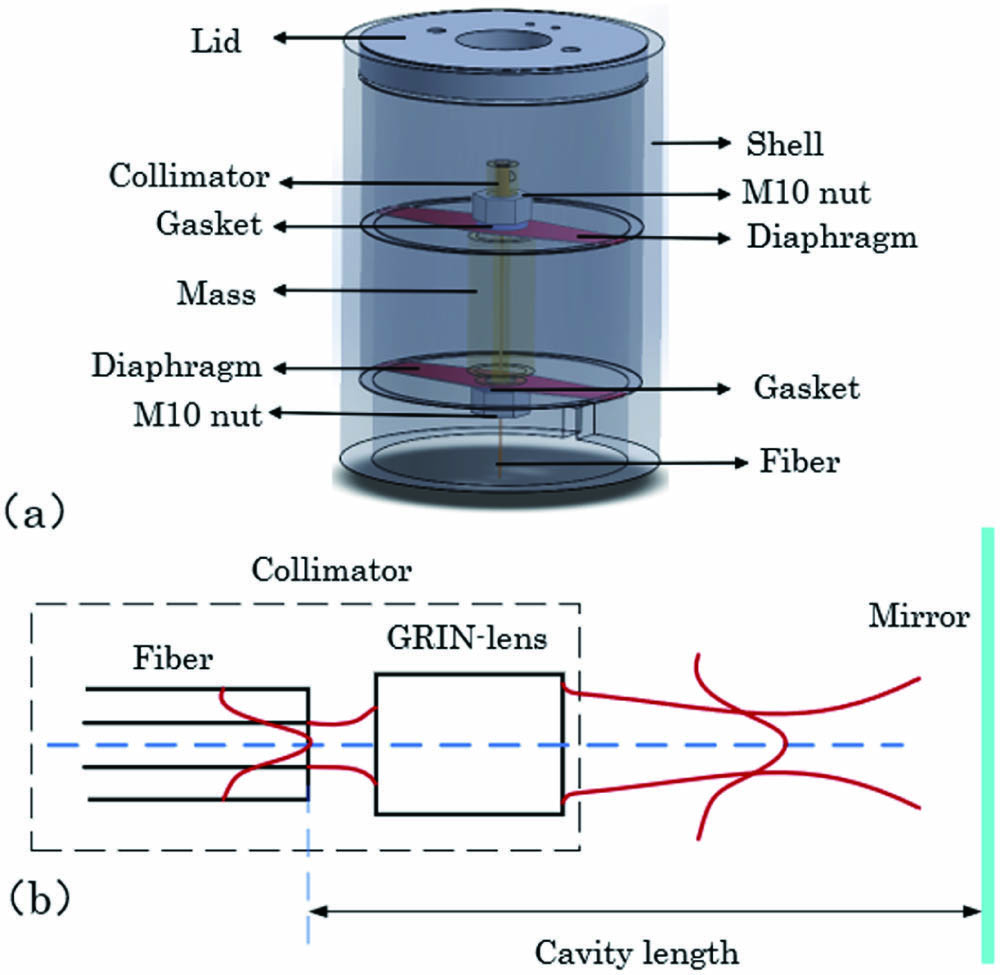
The configuration of the F-P seismometer is shown in Fig. 1. The double-diaphragm sensitization structure is used to reduce the lateral interference, which is fixed at the ends of the mass by gaskets and M10 nuts. The graded-index (GRIN) lens collimator is facing up and fixed in the mass to improve the consistency and make it more compact. The lid is designed as a “skylight” with a trimmer. The mirror is mounted on a trimmer, which is located on the opposite face of the collimator. Since the GRIN lens has an anti-reflection end face, the fiber F-P interferometer is composed by the faces of the fiber and the mirror.

When the F-P seismometer is enacted by ground acceleration, the mass block vibrates up and down, which makes the deflection of the diaphragm change and the collimator motile. The displacement of the collimator changes the interference signal. The acceleration of ground motion and the position of mass are obtained interferometrically by the phase generated carrier (PGC).

The seismometer can be considered as an equivalent second-order vibration system. Figure 2 shows the mechanical model, where y(t) is the displacement of the seismometer relative to the ground reference frame, x(t) is the displacement of the inertial mass relative to the shell of the seismometer, c is the damping coefficient, and K is the equivalent elastic coefficient of the double diaphragm. The relationship between the two can be described by a second-order differential equation, x¨+2ξω0+ω02x=−y¨,(1)where ξ=c/(2mK) is the damping ratio; ω0=K/m is the angular frequency; m is the effective mass of the inertial mass, diaphragms, and collimator.

For the F-P seismometer, the diaphragms are designed as nearly rectangular. Considering the integral method and the principle of small deflection^[14], the equivalent elastic coefficient K can be expressed as K=32Ebh3l3+16r3−12r2l,(2)where l,b,h are, respectively, the length, width, and thickness of the rectangular diaphragms; E is Young’s modulus of the diaphragms; r is the contact radius of the mass and the diaphragm.

The important parameters are given in Table 1, which can be used to design the mechanical structure.

For the F-P interferometer, when the cavity length changes due to the vibration of the mass, the phase change of the interference in the F-P cavity is^[15]Δφ=4πn0ΔLλ,(3)where n0 is the refractive index of air in the F-P cavity and is set as one; λ is the wavelength of the laser beam; ΔL is the cavity length change of the F-P cavity, namely the central deflection of the diaphragm.

Combining Eqs. (1) and (3), the transfer function describes the input–output relationship between the ground acceleration and the phase change, given as H(ω)=S01[1−(f/f0)2]2+(2ξf/f0)2,(4)where f is the frequency of the ground acceleration; f0 is the resonant frequency of the seismometer; S0 is the static sensitivity, indicating the ratio of the phase change to the change of ground acceleration under the steady state condition, and its expression is S0=πm(l3+16r3−12r2l)8λEbh3.(5)

A good seismometer is expected, whose noise level is lower than that of NLNM for low noise measurement. To achieve it, the transfer function of the phase change and the acceleration is separated, and the MDS of the two is used to express it. Here, we assume that the acceleration noise spectrum of the seismometer is equal to the NLNM and assess at what level the resonant point of the seismometer will satisfy the laboratorial demodulation. The MDS xNLNM corresponding to NLNM aNLNM and the MDS xdemodulation corresponding to the demodulation accuracy φdemodulation of our laboratory are, respectively, xNLNM=aNLNM(ω02−ω2)2+(2ξω0ω)2,(6)xdemodulation=φdemodulationλ4π.(7)

The estimation of the MDS, which combines the noise level of instrument requirements and demodulation accuracy, can be used to design the resonant point of the fiber optic seismometer to achieve low frequency observation, as shown in Fig. 3. Note that λ=1550nm and ξ=0.45 are assumed. It can be found that to achieve the acceleration noise less than that of NLNM in the frequency response range above 0.01 Hz, the resonant point should be designed to be less than 1 Hz, which means that the seismometer needs a free period of more than 1 s.

The MDS we presented is not limited to fiber optic F-P seismometers or optical seismic systems described by the transfer function of Eq. (4). According to the noise requirement of the seismometer and the accuracy of the demodulation system, the resonant frequency is designed by optimizing the appropriate mechanical structure.

The MDS described by Eq. (7) is the transfer function between demodulation accuracy and mass position. For the fiber F-P interferometer, the demodulation accuracy and detection threshold are affected, respectively, by the fringe visibility and interference intensity. To achieve high accuracy of the demodulation system, the optical coupling theory is presented to describe each light loss, in which the laser beam is emitted from the fiber core of the collimator, reflected by the mirror, and recoupled to the core.

The F-P interferometer is a multi-beam interference device whose interference intensity and fringe visibility are, respectively, expressed as^[16] IR=R1+ηR2−2ηR1R2cos(4πLλ)1+ηR1R2−2ηR1R2cos(4πLλ)I0,(8)V=2ηR1R2(1+ηR1R2−R1−ηR2)R1+ηR2+ηR12R2+R1(ηR2)2−4ηR1R2,(9)where R1 is the reflectivity of the fiber surface in the collimator due to the Fresnel reflection, R1=0.04; R2 is the mirror reflectivity; I0 is the intensity of the laser beam; η is the coupling efficiency of the F-P cavity; L is the cavity length.

There are main coupling mismatch losses and reflection loss in the F-P cavity. The coupling mismatch losses determined by the mismatch between the collimator and the mirror include axial coupling, lateral coupling, and angular coupling. The reflection loss is caused when light is reflected in the fiber surface. Considering that the light is a Gaussian beam, the expressions of axial coupling, lateral coupling, angular coupling, and reflection loss are, respectively^[17], η1=4(ε2+1)(ε2+2)2,(10)η2=exp[−(nGAπx0s0λ)2],(11)η3=exp[−(θnGAs0)2],(12)η4=16K2(1+K)4,(13)where ε=nG2πs02d/λ, K=n1/n0, s0 is the mode field radius; θ is the tilt angle of the mirror; nG is the central refractive index of the self-focusing lens; A is the focusing constant of the self-focusing lens; x0 is the lateral deviation distance; d=2L is the optical path of a round trip in the F-P cavity; n1 is the core refractive index; n0 is the air refractive index.

Because it is difficult for the fiber surface and the mirror to be strictly parallel in the actual process, when the mirror is tilted, angular coupling generates, which is satisfied by x0/L=tanθ≈θ according to the geometric relationship.

The coupling efficiency of light in the F-P cavity is the superposition of various losses, which is expressed by η=η1×η2×η3×η42.(14)

It can be found that the coupling efficiency is a function of the tilt angle and cavity length. The coupling mismatch losses in the F-P cavity increase with cavity length or tilt angle. When the cavity length is zero, the losses are reflection loss and mismatch loss of angular coupling.

Further combining Eqs. (8) and (9) and assuming the tilt angle, the interference intensity and the fringe visibility of the fiber F-P seismometer can be evaluated.

Figure 4 shows the interference normalized intensity is a function of the cavity length and the mirror reflectivity and indicates that the interference signal intensity decreases with the increase of the cavity length. The reason is that the mismatch losses, including the axial coupling and the lateral coupling, increase with the cavity length. Obviously, the intensity increases with mirror reflectivity.

Figure 5 shows the fringe visibility under different cavity lengths and different mirror reflectivities. When the product of the mirror reflectivity and the coupling efficiency related to cavity length is greater than the reflectivity R1, the fringe visibility increases first and then decreases with the increase of the cavity length. Conversely, the fringe visibility decreases directly.

For further analysis, the reflectivity of the fiber surface and the tilt angle can be designed as other values. The results are similar to the relationships we give in Figs. 4 and 5, which show that the optical coupling theory can be applied to any F-P interferometer composed with a commercial collimator. The theory can improve the signal-to-noise ratio and reduce demodulation noise.

Based on the transfer function analysis of the fiber F-P seismometer, the prototype of the F-P seismometer we proposed had been built. To study the performance of the prototype, the experiment setup shown in Fig. 6 is established. The dashed box is the PGC demodulation system. The modulation frequency is set to 500 Hz, and the modulation voltage is 5.2 V. The 1550 nm laser beam is provided by E15, NKT Photonics. The seismometer is fixed to a vibrator with clamps, and a single mode fiber is connected to the circulator. A standard piezoelectric accelerometer (BK4371) is installed as a reference. In experiments, the distance between the fiber surface and the mirror cavity is about 25 mm. The mirror reflectivity adopted in this prototype is 0.96.

To suppress the environmental noise interference and maintain a relatively constant temperature, the test was done in the super clean room. A 10-cm-thick stainless steel vacuum tank is used to isolate the vibration.

The system is set to calculate once per second, and the fringe visibility of the F-P seismometer is shown in Fig. 7. It can be seen that the fringe visibility corresponding to the F-P seismometer with a cavity length of 25 mm is 0.3, which is close to 0.36 of the simulation in Fig. 5.

We sampled the interference fringe signal and collected 500 samples/s of phase drift to record the phase noise in the time domain of the F-P seismometer in 1345 s. The Pwelch function in MATLAB is used to obtain the power spectral density (PSD) of phase noise in the frequency domain, as shown in Fig. 8. The phase root mean square noise falls from −40dB at 0.01 Hz to −100dB at 10 Hz.

To obtain the acceleration noise, the transfer function [Eq. (4)], which shows a relationship of the phase change and the ground acceleration, is fitted. The polynomial fitting is used to model the transfer function obtained by the experiment. Figure 9 shows the effect of such fitting.

The phase noise is converted into acceleration noise by the fitted transfer function, as shown in Fig. 10. It can be seen that the noise level of the F-P seismometer is much higher than that of NHNM under 0.1 Hz. The main noise limitation factors are resolution of the demodulation system, laser frequency noise, and unavoidable thermal noise. Within the frequency response range of 0.16–50 Hz, the noise level of the F-P seismometer is lower than that of NHNM; as the frequency increases, it approaches NLNM.

One of the potential advantages of the fiber optic F-P seismometer we proposed is that the average noise level is about −143.6dB within 1–50 Hz, which means that the seismometer has a low noise of 6.74ng/√Hz. Within 0.16–1 Hz, the noise level of the F-P seismometer decreases from −105dB at 0.16 Hz to −134dB at 1 Hz, with considerable potential in low frequency seismic monitoring.

In conclusion, we built a fiber optic F-P seismometer prototype based on transfer function analysis, which can achieve low noise measurement in low frequency response. The transfer function of the F-P seismometer is divided, and the method of MDS is introduced to analyze global noise level (or the noise limitation the seismometer required) and demodulation accuracy. The MDS shows that the low frequency monitoring of earth noise can be realized by reducing the resonant frequency and improving the interference fringe. The experiment results show that the PSD of acceleration noise decreases from −105dB at 0.16 Hz to −134dB at 1 Hz, with an average low noise of 6.74ng/√Hz within 1–50 Hz. There is no doubt that the F-P seismometer can measure the local and regional seismic signals of short period frequency band, as well as the remote seismic signal of the medium and short periods.

References

[1] W. Zhang, W. Huang, L. Li, W. Liu, F. Li. High resolution strain sensor for earthquake precursor observation and earthquake monitoring. Sixth European Workshop on Optical Fibre Sensors(2016).
[3] F. Zhang, S. Jiang, X. Zhang, Z. Sun, X. Liu, C. Wang, J.-S. Ni. High resolution 3C fiber laser micro-seismic geophone array for cross-well seismic. AOPC 2017: Fiber Optic Sensing and Optical Communications(2017).
[6] D. Yi, X. Qiu, L. Gu, M. Zhang. Research on an optimized optical fiber accelerometer for well logging. Fiber Optic Sensors and Applications(2017).
[8] Z. Sun, M. Li, S. Jiang, M. Wang, L. Zhang, X. Zhang, C. Wang, Z. Zhao, G. Hao, G. Peng. A high sensitivity fiber Bragg grating seismic system and oil exploration test. 2017 International Conference on Optical Instruments and Technology Advanced Optical Sensors and Applications(2017).
[10] G. H. Ames, J. M. Maguire. Erbium fiber laser accelerometer. IEEE Sens. J., 7, 557(2007).
[14] S. Timoshenko. Theory of Plates and Shells(1964).
[17] X. Lin. Optical Passive Devices(1998).
Set citation alerts for the article
Please enter your email address
© Copyright 2018-2021 | Chinese Laser Press. All Rights Reserved 沪ICP备15018463号-20