
Chuan NONG, Qiu YIN, Ci SONG, Jiong SHU. Sensitivity analysis of the satellite infrared hyper-spectral atmospheric sounder GIIRS on FY-4A[J]. Journal of Infrared and Millimeter Waves, 2021, 40(3): 353
- Journal of Infrared and Millimeter Waves
- Vol. 40, Issue 3, 353 (2021)
Abstract
Keywords
Introduction
From filter to grating and interference(Optical splitting method), the number of channels for atmospheric vertical distribution detection has increased from dozens to hundreds or even thousands [
The instrument noise sensitivity is an important performance index of remote sensor. This index is usually tested in laboratory before launched. When a satellite IHAS is putting into orbit operation, the changes of atmosphere and surface characteristics will affect its output signal.
In this paper, we extend the instrument noise sensitivity concept of the IHAS, put forward the concepts of the atmospheric parameter sensitivity and the surface temperature error sensitivity, introduce their calculation models, and apply them to evaluate the sounding sensitivity of FY-4A GIIRS. The research lays a foundation for the sounding signal-to-noise ratio(SNR) evaluation of atmospheric parameters at different spectral channels.
1 Infrared atmospheric sounding equation
When radiation transfer in the earth-atmosphere system, the atmosphere and the surface may absorb, emit and scatter radiation. The atmospheric molecular scattering and surface reflection are usually neglected for the medium and long wave infrared bands. It is assumed that radiation transfers process is not disturbed by sunlight, the atmosphere is a cloudless, plane-parallel and non-scattering medium with local thermal balance, and the surface is a black body. Taking the viewing direction to the sub-satellite point as the reference, the radiation signal received by the satellite sounder can be written as [
where
According to
We use
where,
If
where,
For an infrared hyper-spectral atmospheric sounder, if there are X detection channels in total and their central wavenumbers are
2 Sensitivity definitions and their calculation models
2.1 Sounder noise sensitivity
The noise sensitivity of infrared sounder is usually characterized by noise equivalent power
where
where
These two indexes are calibrated with the black body whose temperature is adjustable. The results must be noted with conditions of black body temperature and wavenumber.
Supposing the
where,
If the radiant power refers to the power through unit area within unit wavenumber interval and unit solid angle range, then according to Planck’s law of black body radiation, it can be proved
where C1 and C2 are radiation constants. Therefore,
2.2 Atmospheric parameter sensitivity
If the estimated average state of atmospheric parameters and their RMS changes relative to the average state have been known by the statistical analysis of historical data, we can describe the atmospheric parameter sensitivity by the sensitivity of single atmospheric parameter, the comprehensive sensitivity of multiple atmospheric parameters, and the total sensitivity of atmospheric parameters.
(1)The sensitivity of single atmospheric parameter
We define the sensitivity of an atmospheric parameter as the RMS change of sounder received signal caused by the variation of this atmospheric parameter relative to its average state.
If the RMS variation of the kth atmospheric parameter
where,
Supposing that under the conditions of surface temperature
Thus, the sensitivity of the
In section 4, the serial number of atmospheric parameters is directly replaced by name of the atmospheric parameter. For example, atmospheric water vapor sensitivity and atmospheric temperature sensitivity characterized by equivalent temperature difference are written as
(2)The comprehensive sensitivity of multiple atmospheric parameters
We define the comprehensive sensitivity of multiple atmospheric parameters as the RMS change of sounder received signal caused by the variations of several atmospheric parameters.
Supposing that the combined effect of L atmospheric parameters
where,
In other words, the comprehensive sensitivity of several atmospheric parameters is the root of quadratic sum of their respective sensitivities.
If there is a set of atmospheric parameters as the inversion factors and the other atmospheric parameters as the interference factors, the comprehensive sensitivity of former is called the atmospheric target sensitivity and that of the latter is called the atmospheric interference sensitivity.
(3)The total sensitivity of atmospheric parameters
The total sensitivity of atmospheric parameters refers to the comprehensive sensitivity of all atmospheric parameters. If the total sensitivity of atmospheric parameters is expressed by the equivalent power
where,
Obviously, the square of total sensitivity of atmospheric parameters equals the quadratic sum of the atmospheric target sensitivity and its corresponding atmospheric interference sensitivity.
If the atmospheric parameter sensitivity is represented by the equivalent temperature difference instead of the equivalent power,
2.3 Surface temperature error sensitivity
The surface temperature error sensitivity is defined as the RMS change of sounder received signal caused by the estimate error of surface temperature.
If the surface temperature has been determined by some methods such as infrared imager with an accuracy(RMS error) of
where,
If the surface temperature error sensitivity is represented by the equivalent temperature difference
3 Data sources
3.1 FY-4A GIIRS test data
The sensitivity analysis is conducted for FY-4A GIIRS. FY-4A GIIRS is a Fourier spectrometer equipped with infrared focal plane sounder[
3.2 Other data
Atmospheric temperature profile, water vapor profile and ozone profile are obtained from the global reanalysis product ERA-Interim(http://apps.ecmwf.int/datasets/) of ECMWF(European Centre for Medium-Range Weather Forecasts). The product contains 38-year data(1979~2016) in geographical range from 20°E to 180°E and from 80°S to 80°N with 2.5°×2.5° spatial resolution. There are 10512 grid points and 37 layers in vertical direction from 1 000 hPa to 1 hPa.
We use the monthly averaged global atmosphere data to analyze the spatial and temporal changes of atmospheric temperature, water vapor and ozone. The global spatial and temporal changes of these atmospheric parameters in a month are dominated by the spatial change. Taking January 1979 and July 2016 as examples, whether the temporal variation in a month is taken into account leads to a RMS relative difference of 3.92%(Jan 1979)/ 1.97%(July 2016) for evaluating the standard deviation profile of atmospheric temperature from 1hPa to 1 000 hPa. As for atmospheric water vapor and atmospheric ozone, the RMS relative difference are 12.17% /10.25% and 4.90% /6.12% respectively. Taking the month to month variation in one year and the year to year variation in 38 years into account, the overall relatively errors caused by applying monthly averaged global data are under several percent.
The average profiles and the standard deviation profiles of these three atmospheric parameters are calculated. The results for atmosphere temperature have been published[
According to 2017 WMO(World Meteorological Organization) greenhouse gas bulletin[
3.3 Data application method
The sounder received radiation intensity is calculated by the Line-by-Line Radiative Transfer Model(LBLRTM), which is an accurate line-by-line integral calculation program[
For details, the reference atmosphere state and the variation distribution of atmosphere state in
All sensitivity indexes are represented by the equivalent temperature differences.
4 Results
4.1 Sounder noise sensitivity
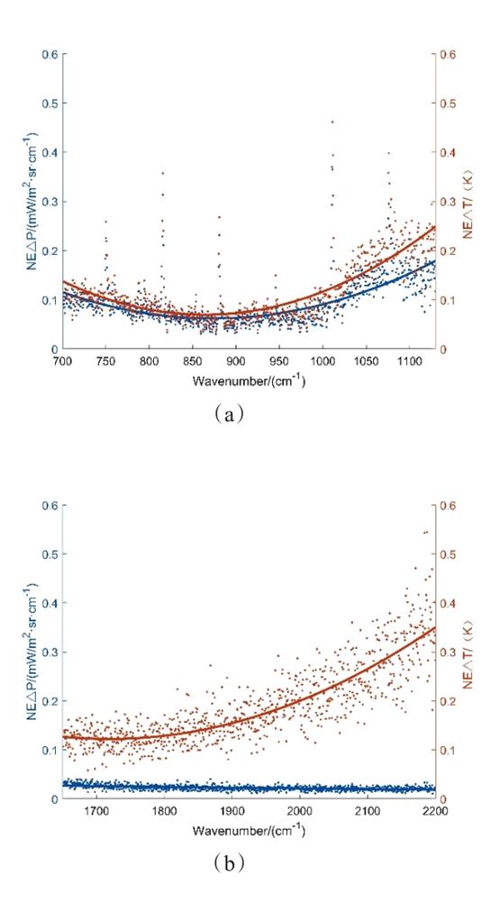
In the laboratory test of FY-4A GIIRS noise sensitivity, the black body temperature is set to 300 K, and the optical interference signal is recorded under this radiation source condition. By means of Fourier inversion, the output spectral response to the input black body radiation is determined, from which the noise equivalent power of each channel is extracted.
The test result of
![]()
Figure 1.The FY-4A GIIRS sounder noise sensitivity @300K for (a) long-wave band and (b) medium-wave band
1) There are some channels in long-wave band, their
2) Excluding these channels with abnormal noises from the sounder noise sensitivity test data, the basic trend of
3) There are no abnormal sensitivity channels in the medium-wave band.
4) In the medium-wave band, the
5) The
4.2 Atmospheric component sensitivity
4.2.1 Atmospheric water vapor sensitivity
Atmospheric water vapor has 6.3 μm absorption band, ranging from 1 200 cm-1 to 2 000 cm-1. Continuous absorption of water vapor exists in the atmospheric window 800-1 200 cm-1. The calculated results of water vapor sensitivity for FY-4A spectral channels are shown in
![]()
Figure 2.The change of atmospheric water vapor sensitivity
| 700~800 | 4.67 | 0.00 | 4.04 | 0.80 |
| 800-1 050 | -1.08 | 4.04 | 0.94 | 0.44 |
| 1 050-1 130 | 0.84 | 0.94 | 1.65 | 0.76 |
Table 1. The statistical characteristics of water vapor sensitivity
| 1 650~2 000 | - | - | - | 4.60 | 1.36 |
| 2 000-2 200 | -1.49 | 3.50 | 0.52 | - | 1.21 |
Table 2. The statistical characteristics of water vapor sensitivity
![]()
Figure 3.Atmospheric water vapor sensitivity
It can be seen from Figs.
1)The variation trend of water vapor sensitivity in long-wave band
The water vapor continuous absorption in 8~14 μm band makes the water vapor sensitivity increasing from 0.94 K @ 1 130 cm-1 to 4.75 K @ 700 cm-1. However, due to the strong absorption of CO2 at 15 μm band, the water vapor sensitivity decreases rapidly from 4.04 K @800 cm-1 to about zero @ 700 cm-1. As can be seen from
2)The variation trend of water vapor sensitivity in medium-wave band
The water vapor absorption at 6.3 μm band makes the water vapor sensitivity of 1 650-2 000 cm-1 high with an average value of 4.60 K. The water vapor sensitivity decreases rapidly from 2 000 cm-1 to 2 200 cm-1. The strong ozone absorption at 4.75 μm band and the CO2 absorption at 5 μm band strengthened the decreasing process.
3)Comparison of the water vapor sensitivity between long-wave band and medium-wave band
The water vapor sensitivity of long-wave channels near 800 cm-1 and that of medium-wave channels in 1 650-2 000 cm-1 is high with average values of 4 K and 4.6 K respectively. The water vapor sensitivity dispersion of medium-wave channels is greater than that of long-wave channels with standard deviations of 1.21~1.36 K for medium-wave channels and 0.44~0.80 K for long-wave channels.
In a word, the basic variation trend of atmospheric water vapor sensitivity with spectral channels is mainly determined by water vapor absorption. The absorption of other gases in their absorption bands, especially the absorption of ozone and CO2, reduces the water vapor sensitivity.
We figure out explanations as follows:
1) An atmospheric absorbing gas affects sounder received signal by affecting the atmospheric transmittance
2) When there are various kinds of absorption components in an atmosphere layer, the radiation transmittance through this layer is a product of the transmittances of each component. Therefore, if we focus on the sensitivity of a certain absorbing gas, the presence of absorption by other gases reduces its sensitivity. The negative effect of CO2 and ozone absorption on atmospheric water vapor sensitivity is a concrete manifestation of this mechanism.
4.2.2 Atmospheric ozone sensitivity
Different from the water vapor, which is mainly concentrated in the troposphere, atmospheric ozone is mainly concentrated in the stratosphere and only absorbs radiation around a few wavenumbers such as 1 041 cm-1 etc. The calculated results of its sensitivity for FY-4A GIIRS spectral channels are shown in
![]()
Figure 4.The change of atmospheric ozone sensitivity
As shown in the
The ozone is most sensitive in its 9.6 μm absorption band. For the wavenumber range of 1 000~1 068 cm-1, the maximum ozone sensitivity is 7.72 K and the average ozone sensitivity is 4.78 K. There is an absorption band near 4.75 μm with a sensitivity of 2.45 K @ 2 018 cm-1. In addition, there is also an absorption band near 700 cm-1.
4.2.3 The sensitivity of atmospheric CO2, N2O and CH4
Significantly different from the vertical and temporal variations of water vapor and ozone, CO2, N2O and CH4 are uniformly distributed and stable in the troposphere and stratosphere.
In the FY-4A GIIRS wavenumber range, CO2 has a strong 15 μm absorption band. There are also absorption bands of CO2 near 10.6 μm and 5 μm. N2O only has a 4.5 μm absorption band, and CH4 has no significant absorption band, only very weak absorption around 7.7 μm.
The sensitivity variations of these trace gases with the FY-4A GIIRS channels are shown in Figs.
![]()
Figure 5.The change of atmospheric CO2 sensitivity
![]()
Figure 6.The change of atmospheric N2O sensitivity
![]()
Figure 7.The change of atmospheric CH4 sensitivity
It can be seen from the figures that although CO2 has several absorption bands such as 15 μm strong absorption band, its sensitivity is much smaller than that of water vapor and ozone due to its stability. The maximum sensitivities of water vapor and ozone are 6.41 K and 7.72 K respectively, while the maximum sensitivity of CO2 is only 0.09 K. Similarly, N2O only has the maximum sensitivity at the high wavenumber end of the medium-wave band, which is only 0.04 K. As for CH4, the sensitivity is even lower.
4.3 The atmospheric temperature sensitivity
![]()
Figure 8.The change of atmospheric temperature sensitivity
![]()
Figure 9.Atmospheric temperature sensitivity
As can be seen from
However, there are other absorbing gases such as ozone, CO2, N2O and CH4 in actual atmosphere. As can be seen from
Similarly, for 2 000~2 200 cm-1 in the medium-wave band, the atmospheric temperature sensitivity also increased due to the presence of ozone, CO2 and N2O absorption. Atmospheric temperature sensitivity increases from an average of 5.32 K(standard deviation 3.81 K) in the case of only water vapor to 7 K(standard deviation 3.34 K).
In summary, water vapor absorption determines the basic state of atmospheric temperature sensitivity, and the presence of other absorbing gases increases the atmospheric temperature sensitivity at their absorption bands.
By comparing effects of these absorbed gases on water vapor sensitivity, their effects on atmospheric temperature sensitivity are opposite to their effects on water vapor sensitivity.
Atmospheric temperature sensitivity is positively correlated with water vapor and other gas absorption. As shown in the infrared atmospheric sounding equation
4.4 Surface temperature error sensitivity
The variation of surface temperature error sensitivity with FY-4A GIIRS spectral channels is shown in
![]()
Figure 10.The change of surface temperature error sensitivity
| 700-750 | 0.04 | 0.07 |
| 750-800 | 0.44 | 0.21 |
| 800-1 000 | 0.74 | 0.13 |
| 1 000-1 068 | 0.50 | 0.17 |
| 1 068-1 130 | 0.80 | 0.16 |
Table 3. The statistical results of the surface temperature error sensitivity
| 1 650-1 900 | 0.01 | 0.01 |
| 1 900-2 000 | 0.14 | 0.18 |
| 2 000-2 200 | 0.53 | 0.28 |
Table 4. The statistical results of the surface temperature error sensitivity
It can be seen from
The reason is that, as shown by section 4.3, the stronger the atmospheric absorption is, the higher the atmospheric temperature sensitivity will be. On the contrary, according to the infrared atmospheric sounding equation
4.5 The comparison of different sensitivity indices
By comparing the sensitivity characteristics of atmospheric absorbing gases, atmospheric temperature and surface temperature error, we can see that:
1) The sensitivity of atmospheric water vapor and ozone are generally at levels of several degree(K), and the maximum value of the former and the latter are 6.41 K and 7.72 K respectively. The sensitive wavenumber range of ozone is limited to a narrow absorption bands such as 9.6 μm, while water vapor has a wide sensitive wavenumber coverage.
2) The sensitivity of CO2 and N2O are all below 0.1 K, and sensitivity of CH4 is closer to zero. The reason is that these trace gases are very stable compared with water vapor and ozone.
3) Similar to atmospheric water vapor, atmospheric temperature has a wide sensitive wavenumber coverage, and its overall level of sensitivity is higher than that of water vapor and ozone with maximum value of 14.30 K.
4) The surface temperature error sensitivity is generally at a level of tenths degree with maximum of 0.93 K. Its variation characteristics is opposite to that of atmospheric temperature sensitivity.
5) The equivalent temperature difference of sounder noise follows the sounder itself, which varies in range of 0.04 ~ 0.54 K. As disturbing factors, contribution of the surface temperature error is generally higher than that of sounder noise, and the contributions of CO2, N2O and CH4 are much less than that of surface temperature error and sounder noise.
5 Summary
In this paper, the sensitivity concept of infrared hyper-spectral atmospheric sounder is extended to atmospheric parameter sensitivity and surface temperature error sensitivity for the on-orbit application of satellite sounder. The sensitivity calculation models and their relations for different indices of atmospheric parameter sensitivity are established. The relations between equivalent power and equivalent temperature difference expressing sensitivity indices are introduced.
The sounder noise sensitivity, the sensitivity of different atmospheric parameters, and the surface temperature error sensitivity are evaluated and analyzed FY-4A GIIRS. The main conclusions are as follows:
1) The
2) The sensitivities of atmospheric water vapor and that of ozone are at the same level of several degree, which is lower than that of atmospheric temperature whose maximum is about 14.3 K. The sensitive channels of atmospheric water vapor and atmospheric temperature covers wide wavenumber range, while the sensitive channels of ozone are limited to a few very narrow absorption bands.
3) The sensitivity of CO2 and N2O are all below 0.1 K and the sensitivity of CH4 is close to zero, which is much lower than that of atmospheric water vapor and ozone.
4) The surface temperature error sensitivity is generally at level of a few tenths with maximum of 0.93 K. Its variation characteristic with spectral channels is opposite to that of atmospheric temperature sensitivity.
The physical mechanisms of the sensitivity evaluation results are analyzed. The main conclusions are as follows:
1) The sensitivity of an atmospheric gas is positively correlated with its own absorption strength, and negatively correlated with the absorption strengths of other atmospheric gases.
2) The sensitivity of atmospheric temperature is positively correlated with the absorption strength of every absorbing gas, while the sensitivity of surface temperature error is negatively correlated with the absorption strength of every absorbing gas.
3) The sensitivity of CO2, N2O and CH4 are far lower than other atmospheric parameters, due to their contents in atmosphere are very stable.
In the follow-up works, we will analyze the signal-to-noise ratios of atmospheric temperature, water vapor and ozone by satellite infrared hyper-spectral sounding, so as to achieve the primary selection of sounding channels.
References
[4] Y S. Bao, Z J Wang, Q Chen et al. Preliminary study on atmospheric temperature profiles retrieval from GIIRS based on FT-4A satellite. Aerospace Shanghai, 34, 28-37(2017).
[5] Yao-Hai Dong. FY-4 meteorological satellite and its application prospect. Aerospace Shanghai, 33, 1-8(2016).
[8] Liou Kuo-Nan. An Introduction to Atmospheric Radiation(2004).

Set citation alerts for the article
Please enter your email address
© Copyright 2018-2021 | Chinese Laser Press. All Rights Reserved 沪ICP备15018463号-20