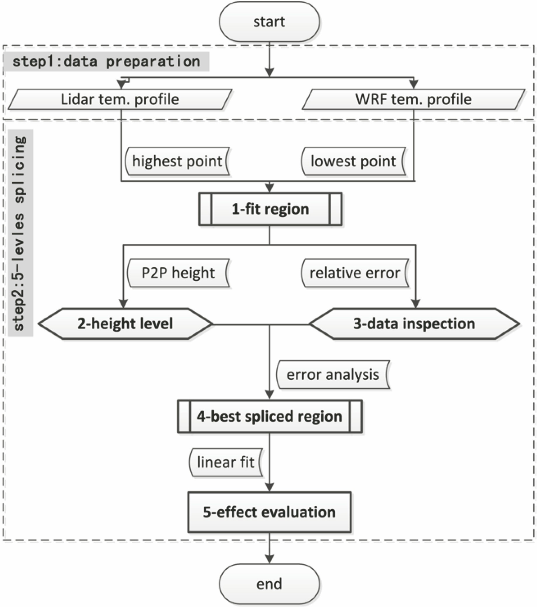
Fig. 1. Flow chart of data splicing

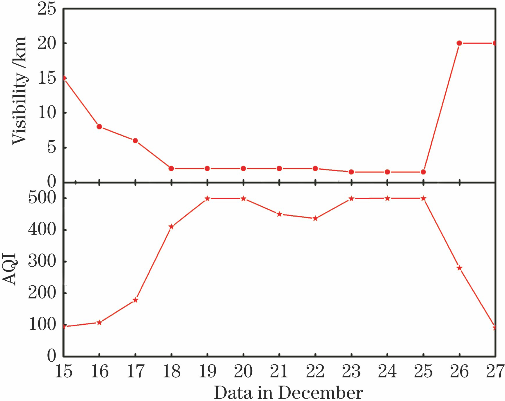
Fig. 2. Visibility and AQI before and after the typical fog-haze case in Xi'an

Fig. 3. Qualitative analysis of the temperature profile during model data, lidar data and radiosonde data. (a) <2 km; (b) 2~20 km

Fig. 4. Quantitative analysis of the splicing data and radiosonde data on relative error. (a) Between lidar data and radiosonde data; (b) between model data and radiosonde data

Fig. 5. Relative error corresponding to 11 groups of step sizes

Fig. 6. Judgment criteria for based on 20 groups of splicing-regions in 4 groups of samples. (a) Correlation coefficient; (b) splicing-region deviation per km

Fig. 7. Parameters for selecting the best splicing-region. (a) Correlation coefficient; (b) splicing-region deviation per km; (c) fit-region deviation per km

Fig. 8. Temperature splicing results between model and lidar data. (a) Qualitative contrast on profiles between splicing temperature and standard temperature during the whole layers; (b) quantitative contrast on relative error between splicing temperature and standard temperature during the whole layers; (c) qualitative contrast on profiles between splicing temperature and standard temperature in the best splicing region

Fig. 9. Temperature splicing results between radiosonde and lidar data, and their comparison with the splicing results between model and lidar data. (a) Profile of splicing temperature between radiosonde and lidar data during the whole layers; (b) qualitative contrast on profiles between radiosonde-lidar splicing temperature and standard temperature in the best splicing region; (c) quantitative contrast on relative errors between the model-lidar splicing temperature and standard temperature, and between

Fig. 10. Splicing-region deviation per km corresponding to 8 groups of splicing-regions to be selected

Fig. 11. Contrast of splicing temperature at 20:00 UTC during the whole fog-haze phase. (a) Unsplicing temperature profile. (b) splicing temperature profile

Table 1. Parameters for WRF model simulation

Table 2. Comprehensive evaluation parameters between model-lidar splicing and radiosonde-lidar splicing