To describe the measured radiation of infrared targets continuously and accurately, data fitting is necessary for the calibration of the infrared radiometer. Data fitting is essentially a typical function approximation problem. The fitting accuracy will be different owing to the differences between fitting methods, which will influence the measurement accuracy of the infrared radiometer.

In the calibration of the infrared radiometer, the least-squares (LS) method has been most widely used in data fitting^[1-4]. The commonly used approximation function of the LS method is polynomials^[5-10], as well as others such as sinusoidal function and log function^[11-12]. However, the LS method is a global approximation scheme, which is not suitable for irregular or non-uniform distribution cases. For the LS method, the oscillation phenomenon occurs and the oscillation increases dramatically when the order of polynomial becomes larger, which reduces the fitting accuracy. For the calibration of the infrared radiometer, problems observed contain the non-uniform distribution of fitting data, the dramatic change in the order of magnitude, and the limitation on the number of calibration points, which resulting in sufficient fitting precision cannot be achieved by the LS method.

To improve the fitting accuracy, The Adaptive Moving Least Squares (AMLS) method is used in this paper for data fitting in the calibration of the infrared radiometer, which combines Adaptive Processing (AP) and Moving Least Squares (MLS). AP procedures such as data transformation or data translation are performed before the calibration data fitting to reduce the adverse effect resulting from irregular or non-uniform data distribution. The MLS method combines the concept of moving window and compact support weighting functions, which can be regarded as a combination of Weighted Least Squares (WLS) and Segmented Least Square (SLS). As a local approximation method, The MLS method can not only acquire higher precision even with low order basis functions but also has good stability due to its local approximation scheme^[13]. However, the parameters setting in the MLS method are often chosen through individual experience or simple parameters adjustment^[14], by which optimal fitting accuracy is difficult to achieve. Thus, to carry out the optimization mechanism corresponding to the setting of weighting function parameters in the MLS method, the Particle Swarm Optimization (PSO) technique is used with the AMLS method. As a “speed-position” searching algorithm, the particle adjusts its speed vector value and direction following the optimal particle, and then the optimal penalty parameters of samples can be obtained^[15].

In this paper, the hybrid PSO-AMLS-based method is proposed for data fitting in the calibration of the infrared radiometer. The present study is structured as follows: firstly, proposed methods and principles are explained in Section 1; secondly, numerical examples of curve fitting is carried out based on hybrid PSO-AMLS-based method in Section 2, containing the examples when the independent variables are uniform distribution and non-uniform distribution; thirdly, the hybrid PSO-AMLS-based method is applied to the calibration of the infrared radiometer in Section 3; and finally, the main conclusions of this research work are drawn.

As a conventional data fitting method, the MLS method was proposed by Shepard in 1968^[16]. The basic theory of the MLS can be seen in references [17] and [18], so this paper only gives a brief introduction. In MLS, an arbitrary function f(x) can be approximated by

$ f(x) = \sum\limits_{i = 1}^m {{p_i}} (x){a_i}(x) = {P^{\rm T}}(x)a(x) $ (1)

where p_i(x) are basis functions, a_i(x) are the coefficients, the coefficients a(x)=[a₁(x), a₂(x),···, a_m(x)]^T varied with x. In order to determine the coefficients a_i(x), a function is defined as

$ J = \sum\limits_{I = 1}^N {{w_I}} (x){[P({x_I})a(x) - f({x_I})]^2} $ (2)

where f(x_I) are the given nodes, ω(x) is the weighting function with compact support.

One commonly used weighting function is the Gaussian function, which is very flexible for the MLS and is adopted in the following discussion. The Gaussian weighting function is

$ w(r) = \left\{ {\begin{array}{*{20}{c}} {\dfrac{{{\rm exp}( - {r^2}{\beta ^2}) - {\rm exp}( - {\beta ^2})}}{{1 - {\rm exp}( - {\beta ^2})}}{\kern 1pt} {\kern 1pt} {\kern 1pt} {\kern 1pt} {\kern 1pt} {\kern 1pt} {\kern 1pt} {\kern 1pt} {\kern 1pt} {\kern 1pt} r \leqslant 1} \\ {{\kern 1pt} {\kern 1pt} {\kern 1pt} {\kern 1pt} {\kern 1pt} {\kern 1pt} {\kern 1pt} {\kern 1pt} {\kern 1pt} {\kern 1pt} {\kern 1pt} {\kern 1pt} {\kern 1pt} {\kern 1pt} {\kern 1pt} {\kern 1pt} {\kern 1pt} {\kern 1pt} {\kern 1pt} {\kern 1pt} {\kern 1pt} {\kern 1pt} {\kern 1pt} {\kern 1pt} {\kern 1pt} {\kern 1pt} {\kern 1pt} {\kern 1pt} {\kern 1pt} {\kern 1pt} {\kern 1pt} {\kern 1pt} {\kern 1pt} {\kern 1pt} {\kern 1pt} {\kern 1pt} {\kern 1pt} {\kern 1pt} {\kern 1pt} {\kern 1pt} {\kern 1pt} {\kern 1pt} {\kern 1pt} 0{\kern 1pt} {\kern 1pt} {\kern 1pt} {\kern 1pt} {\kern 1pt} {\kern 1pt} {\kern 1pt} {\kern 1pt} {\kern 1pt} {\kern 1pt} {\kern 1pt} {\kern 1pt} {\kern 1pt} {\kern 1pt} {\kern 1pt} {\kern 1pt} {\kern 1pt} {\kern 1pt} {\kern 1pt} {\kern 1pt} {\kern 1pt} {\kern 1pt} {\kern 1pt} {\kern 1pt} {\kern 1pt} {\kern 1pt} {\kern 1pt} {\kern 1pt} {\kern 1pt} {\kern 1pt} {\kern 1pt} {\kern 1pt} {\kern 1pt} {\kern 1pt} {\kern 1pt} {\kern 1pt} {\kern 1pt} {\kern 1pt} {\kern 1pt} {\kern 1pt} {\kern 1pt} {\kern 1pt} {\kern 1pt} {\kern 1pt} {\kern 1pt} {\kern 1pt} {\kern 1pt} {\kern 1pt} {\kern 1pt} {\kern 1pt} r > 1} \end{array}} \right. $ (3)

where r=|x−x_I|/d_mi is the relative distance, d_mi is the influencing radius, and β is the shape parameter.

Then, the matrix form for equation (2) can be rewritten as

$ J = {[Pa(x) - f]^{\rm T}}W[Pa(x) - f] $ (4)

where f =[f (x₁), f (x₂),···, f (x_N)]^T, P and W are

$ P = {\left[ {\begin{array}{*{20}{c}} {{P^{\rm T}}({x_1})} \\ {{P^{\rm T}}({x_2})} \\ \vdots \\ {{P^{\rm T}}({x_N})} \end{array}} \right]_{N \times m}} $ (5)

$ W = \left[ {\begin{array}{*{20}{c}} {\omega (x - {x_1})}&0& \cdots &0 \\ 0&{\omega (x - {x_2})}& \cdots &0 \\ \vdots & \vdots & \ddots & \vdots \\ 0&0& \cdots &{\omega (x - {x_N})} \end{array}} \right] $ (6)

Minimizing equation (4) with respect to coefficients a(x), the following expression can be obtained

$ \frac{{\partial J}}{{\partial a(x)}} = [{P^{\rm T}}WP]a(x) - [{P^{\rm T}}W]f = 0 $ (7)

Further, the coefficients a(x) and function f(x) are obtained as follows

$ a(x) = {[{P^{\rm T}}WP]^{{\rm{ - }}1}}[{P^{\rm T}}WP]f $ (8)

$ f(x) = {P^{\rm T}}(x){[{P^{\rm T}}WP]^{{\rm{ - }}1}}[{P^{\rm T}}WP]f $ (9)

However, the calculation process of the MLS method is more complicated and requires a larger amount of computation.

The PSO technique is a population-based search algorithm based on the simulation of the bird flocking. The basic theory of the MLS can be seen in reference [19], so this paper only gives a brief introduction. In the PSO, the parameters or possible set of solutions are contained in a vector x_i(k), which is called a particle of the swarm and represents its position in the search space of possible solutions. The particle dimension is the number of parameters. The particle initial position x_i(0) and its velocity v_i(0) are chosen randomly. The value of the fitness function is then calculated for each particle and the velocities, and then the positions are updated depending on these values. The algorithm updates the positions and the velocities of the particles as follows:

$ \begin{split} {v_i}\left( {k + 1} \right) =& \omega \cdot {v_i}\left( k \right) + {c_1} \cdot {r_1} \cdot \left( {{p_{ibest}} - {x_i}\left( k \right)} \right) + {c_2} \cdot \\ & {r_2} \cdot \left( {{g_{best}} - {x_i}\left( k \right)} \right) \\ \end{split} $ (10)

$ {x_i}\left( {k + 1} \right) = {x_i}\left( k \right) + {v_i}\left( {k + 1} \right) $ (11)

where ω is the inertia factor, p_ibest is the local best position; g_best is the global best position; c₁ and c₂ are learning factors; rand() is a random number in the interval [0, 1].

The current position x_i(k) and velocity v_i(k) of each particle are adjusted depending on its status in the previous step, the particle’s local best position p_ibest, and the global best position g_best. The particles of the swarm make up a cloud that covers the whole search space in the initial iteration and gradually contracts its size as iterations advance to perform the exploration. So in the initial stages, the algorithm performs an exploration searching for plausible zones, and in the last iterations the best solution is improved^[20]. In this paper, c₁ and c₂ are set to 2, maxgen is set to 120, sizepop is set to 20, ω is set to 1, and v_max is set to 5.

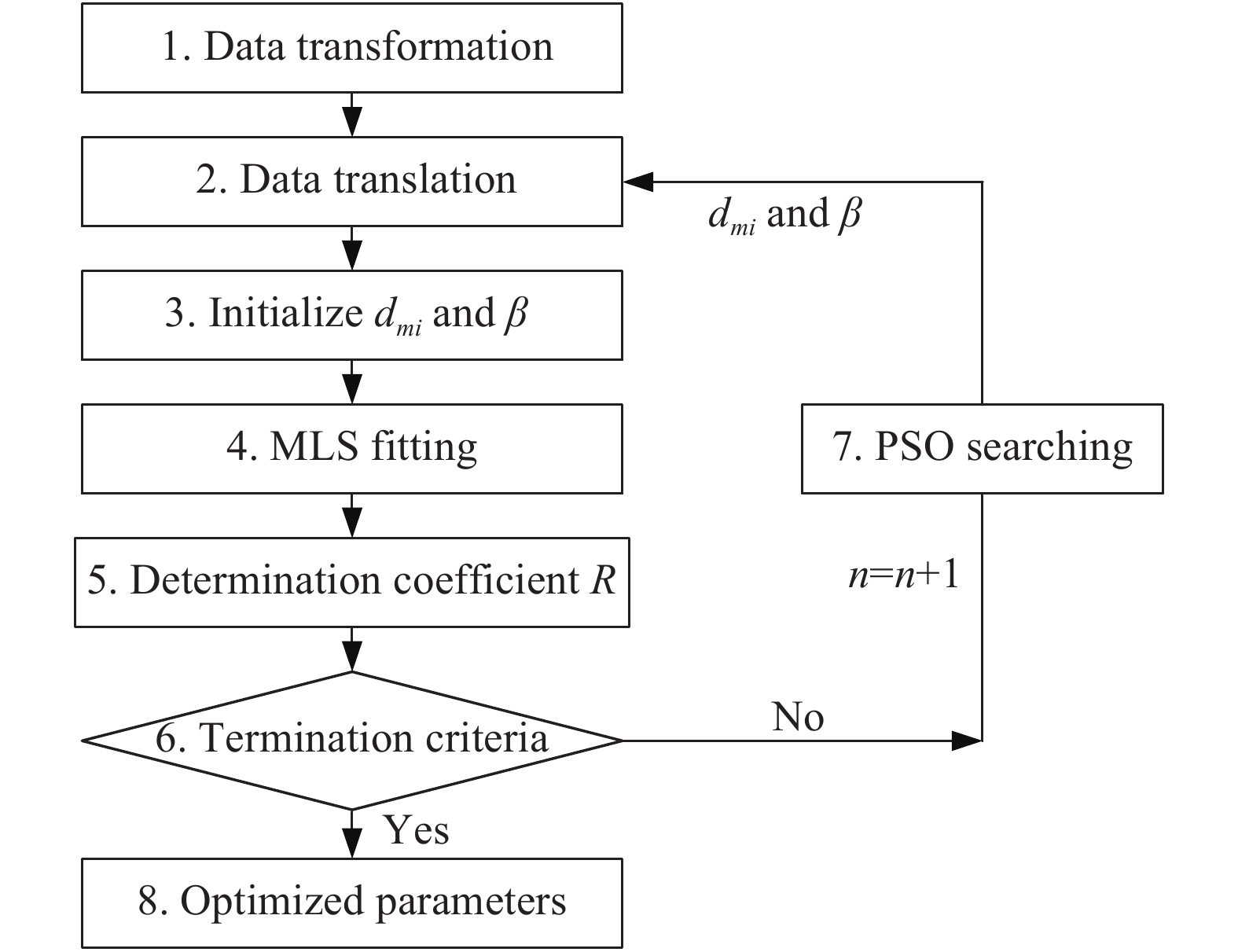
The PSO-AMLS-based method can be regarded as a combination of AP procedures, PSO technique and MLS fitting method. For the implementation of the PSO-AMLS method, firstly, the calibration data is pretreated using AP procedures; secondly, the MLS method is used for the fitting of pretreated calibration data, in which the PSO method is used to carry out the optimization mechanism to get the optical weighting function parameters in the MLS method. The flowchart of the PSO-AMLS-based method is shown in Figure 1. Through adaptive data processing in procedures (1) and (2), possible extreme value, non-normal distribution, or the dramatic change in the order of magnitude can be reduced or eliminated.

For basic functions selection in the MLS, lower-order polynomials are preferred. For parameters setting in Gaussian weighting function, larger influencing radius d_mi means better fitting smoothness; larger shape parameter β means the locality is enhanced while the smoothness is declined. To optimize the MLS parameters, the PSO searches for the best parameters by comparing the fitness factor. The main fitness factor used in this paper is the determination coefficient R², which is defined as follows:

$ {R^2} = \sum\limits_{i = 1}^n {{{\left( {{y_i} - {y_{if}}} \right)}^2}} $ (12)

where y_i is the dependent variable of calibration point, y_if is the fitting value, n is the number of calibration points.

In this Section, numerical examples are carried out to investigate the fitting performance of the PSO-AMLS-based method. Functions similar to the calibration data of the infrared radiometer are used in this section. In the first example, the independent variables are uniform distribution. In the second example, the independent variables are non-uniform distribution. The data were processed in this paper with code written in MATLAB.

The formula used in the first example is as follows:

$ f(x) = 1 + \sqrt x $ (13)

A set of points (x_i, y_i) are chosen, where i=0-20. The independent variables are uniform distribution from 0 to 20 with interval h=1, while the interval of dependent variables is gradually increased and determined by equation (13). The data used in the first example is shown in Table 1.

The Gaussian function is chosen to be the weighting function. Considering the fitting accuracy and oscillation problem, the polynomial order is 6 for the LS method. The fitting performance is characterized by the fitting error δ between real value y_i and fitting value y_if

$ \delta = {y_i} - {y_{if}} $ (14)

The PSO is used to optimize the MLS parameters d_mi, β, and m, where m represents the type of the basic function. The basic function is set to be p₁(x) = [1], p₂(x) = [1, x] and p₃(x) = [1, x, x²] when m=1, m=2 and m=3, respectively. Search space is organized in three dimensions, one for each parameter. Because the independent variables are uniform distribution, there is no AP performed in this example. The fitting errors δ of the LS and PSO-AMLS method when the independent variables are uniform distribution are shown in Figure 2.

The parameter “nnodes” is the number of nodes used in the PSO-AMLS method. For the cases when the independent variables of fitting data are uniform distribution, the PSO-AMLS method can acquire better results than the LS method. The PSO-AMLS method can follow the changes of the original function even with low order basis function, while, for the global approximation scheme like the LS, the oscillation phenomenon occurs, which increases the approximation error. When nnodes is 11, an outlier exists where δ_PSO-AMLS is larger than δ_LS. The position and amplitude of the outlier are x=1 and δ_PSO-AMLS=0.19. According to the amplitude δ, the results when nnodes is 21 are much better than the results when nnodes is 11, fewer nnodes means larger d_mi is needed. When nnodes is too little, the fitting accuracy may be affected; when nnodes is too much, the regional feature may not be obvious but can be enhanced by the adjustment of parameters in the AMLS.

In this subsection, a set of points (x_i, y_i) are used as the calibration points, where i=1-15. The dependent variables are uniformly distributed with interval h=1, while the independent variables are non-uniformly distributed and the intervals are gradually increased. The data used in the second example is shown in Table 2.

The parameters setting in the PSO and the AMLS are the same as in Subsection 3.1. Because the independent variables are non-uniform distribution, logarithmic transformation is performed before the MLS in this example. For the observed fitting results of the LS method are too bad when the independent variables are non-uniformly distribution, the Adaptive Least Squares (ALS) method is used in this subsection to compare with the PSO-AMLS method, where logarithmic transformation is performed before the LS. The fitting errors δ of the ALS and the PSO-AMLS method when the independent variables are non-uniform distribution are shown in Figure 3, in which the x-coordinate is the serial number of points.

It is shown in Figure 3 that, for the cases when the independent variables of fitting data are non-uniform distribution, the PSO-AMLS method can acquire much better results than the LS method. The oscillation phenomenon occurs both for the ALS and the PSO-AMLS method, but the oscillation amplitude of the PSO-AMLS method is much smaller than that of the ALS method. Combined with the results obtained in Subsection 3.1, it is concluded that the fitting performance of the PSO-AMLS method is superior compared to the LS and ALS method.

In this Section, based on the infrared radiometer and the data fitting method described above, the calibration of the infrared radiometer has been carried out. The comparison of different data fitting methods is performed to validate the effectiveness of the PSO-AMLS method in the real calibration.

The response voltages V of the infrared radiometer were measured in the calibration, where a blackbody-collimator was used as the standard source. Figure 4 is a diagram of the infrared radiometer. The basic components of the infrared radiometer are the optical lens, chopper, detector, preamplifier, lock-in amplifier, and A/D.

The main specifications of the infrared radiometer are shown in Table 3. The basic components of the blackbody-collimator are the blackbody, collimator, and aperture. The main specifications of the blackbody-collimator are shown in Table 4. The blackbody temperatures T are uniform distribution from 100 ℃ to 700 ℃ with interval h=50 ℃. The corresponding calibration data of T and V are shown in Table 5.

It is shown from Table 5 that the dependent variables are uniform distribution with equal interval, while the independent variables are non-uniform distribution and the intervals increase gradually. The reasons for this phenomenon are as follows: (1) the response voltage of the infrared radiometer is affected significantly by the standard radiation source; (2) the response of the infrared radiometer is mainly determined by the detection ability of the detector.

For the data characteristic mentioned above and the number limitation of calibration data, conventional data fitting methods commonly used in the calibration of infrared radiometer cannot achieve enough fitting accuracy. The fitting errors δ using the LS method and ALS method are shown in Figure 5. In Figure 5(a), polynomial approximate based on the LS method is carried out with polynomial orders from 5 to 6. In Figure 5(b), logarithmic transformation is carried out before the polynomial approximate with the polynomial orders from 5 to 6.

It can be obviously seen that the ALS method can acquire much better results than the LS method, which means the AP is effective to improve the fitting accuracy and stability when the fitting points are non-uniform distribution. But for the LS and ALS methods, the oscillation phenomenon occurs and the approximation errors change dramatically, especially when the number of calibration points is small and the fitting data are non-uniform distribution.

To improve the fitting accuracy, the PSO-AMLS-based method is applied in the calibration of the infrared radiometer. The fitting errors of the PSO-AMLS method are compared to the ALS method to verify the performance of the PSO-AMLS method. For the PSO-AMLS with LT, only logarithmic transformation is contained in the AP, but for the PSO-AMLS with LT and DT, both logarithmic transformation and data translation are contained in the AP. The fitting errors of the PSO-AMLS and ALS method are shown in Figure 6.

In Figure 6, the R² of the PSO-AMLS method is 1.8437 compared with 3.6962 of the ALS method, which means better fitting results are achieved by the PSO-AMLS method. The superior performance of the PSO-AMLS method is more obvious in the first half of calibration points, while in the second half, an outlier exists in point 10 where δ_PSO-AMLS is slightly larger than δ_ALS, and δ_PSO-AMLS and δ_ALS are almost the same for point 12 and 13. It is supposed that the reason of this phenomenon is the number limitation of calibration points in the second half of the calibration data. Fitting errors δ will be increased when fewer calibration points are used. In the shape function matrix of the PSO-AMLS method, the locality is strong at the beginning, but decline with the increase of voltage. At the end of the calibration points, the locality is weakened but the globality is enhanced. In addition, it is shown that the performance of the PSO-AMLS with LT is only slightly better than the PSO-AMLS with LT and DT, which means the effect of logarithmic transformation is more obvious than data translation in the AP. The PSO-AMLS method should provide a better fitting result but suffer from the number limitation of fitting data, especially in the calibration of the infrared radiometer. As a future line of research, to improve the fitting performance when the samples of fitting data are fewer, more AP methods will be used.

In this section, the infrared radiometer calibrated using different data fitting methods is applied to the measurement of an infrared imaging simulator in the medium waveband. The measurement parameter is the equivalent blackbody temperature. The measured targets include the target channel and the interference channels. The source of target channel and interference channels are high-pressure xenon lamps, and the output radiation is controlled by the adjustment of the working current. The collimator and apertures used in the experiment are the same as in the calibration of the infrared radiometer. The equivalent blackbody temperature T_t measured by the thermal imaging camera ImageIR-5300 is used as the reference value. T_m measured by the infrared radiometer using two fitting methods is compared to the reference value T_tto obtain the deviation δ^*:

$ {\delta ^*} = {T_t} - {T_m} $ (15)

The deviation δ^* obtained for different fitting methods are shown in Figure 7, where TC represents Target Channel, IC 1, 2, and 3 represents Interference Channel 1, 2, and 3.

It is shown from Figure 7 that for different measured targets, the measured T_m for the PSO-AMLS method is closer to the reference value compared to the ALS method. Besides, compared with the measurement results in section 3.1, more error sources are introduced in this measurement, including the repeatability and reproducibility, which results in the unexpected changes of the measured voltage. However, the most important result is that the PSO-AMLS method is more superior compared to other conventional fitting methods, which is effective for the improvement of measurement accuracy of the infrared radiometer.

The hybrid PSO-AMLS-based method was proposed for data fitting in this paper. The superior performance of the PSO-AMLS method was demonstrated by numerical examples and application in engineering. The main findings of this research work can be summarized as follows:

(1) The hybrid PSO-AMLS-based method is successfully applied to data fitting in the calibration of the infrared radiometer. The fitting performance is confirmed by numerical examples and experiments. Compared to the conventional data fitting methods, better fitting results are achieved by the PSO-AMLS-based method;

(2) From the obtained fitting results using the PSO-AMLS method, it is suggested that the use of the MLS approximation in combination with the PSO technique and AP process. In summary, the hybrid PSO-AMLS-based method is a promising method for data fitting, which can be applied to other calibration of instruments with success.

References

[1] A Ville, W B Steven, C L Thomas, et al. Comparison of absolute spectral irradiance responsivity measurement techniques using wavelength-tunable lasers. Applied Optics, 46, 4228-4236(2007).
[2] J Hartmann. High-temperature measurement techniques for the application in photometry, radiometry and thermometry. Physics Reports, 469, 205-269(2009).
[3] Wang X, Gao Z Y, Zhang J Y, et al. Research on calibration method of three b infrared integrated radiometer[C]Proceedings of SPIE, 2002, 4927: 133138.
[4] R Ibrahim, R H John, G Julian, et al. Calibrating pyrgeometers outdoors independent from the reference value of the atmospheric longwave irradiance. Journal of Atmospheric and Solar-Terrestrial Physics, 68, 1416-1424(2006).
[5] S Anevsky, V Krutikov, O Minaeva, et al. Method for the calibration of the spectral irradiance of tungsten filament transfer standard sources traceable to synchrotron radiation. Applied Optics, 52, 5152-5157(2013).
[6] L K Huang, R P Cebula, E Hilsenrath. New procedure for interpolating NIST FEL lamp irradiances. Metrologia, 35, 381-386(1998).
[7] F Samedov, M Durak, O Bazkir. Filter-radiometer-based realization of candela and establishment of photometric scale at UME. Optics and Lasers in Engineering, 43, 1252-1266(2005).
[8] M Durak, M H Aslan. Optical characterization of the silicon photodiodes for the establishment of national radiometric standards. Optics & Laser Technology, 36, 223-227(2004).
[9] H Minato, Y Ishido. Development of a five-band multi-spectral infrared radiometer for low temperature measurements. Review of Scientific Instruments, 74, 2863-2870(2003).
[10] R R Cordero, G Seckmeyer, D Pissulla, et al. Uncertainty evaluation of spectral UV irradiance measurements. Measurement Science and Technology, 19, 045104(2008).
[11] H E Revercomb, H Buijs, H B Howell, et al. Radiometric calibration of IR Fourier transform spectrometers: solution to a problem with the High-Resolution Interferometer Sounder. Applied Optics, 27, 3210-3218(1988).
[12] Flynn D S, Marlow S A, Sisko R B, et al. Accuracy of aperture irradiances from a resistarray projection system[C]Proceedings of SPIE, 2005, 5785: 112123.
[13] H Q Zhang, C X Guo, X F Su, et al. Measurement data fitting based on moving least squares method. Mathematical Problems in Engineering, 2015, 195023(2015).
[14] L Zhang, T Q Gu, J Zhao, et al. An improved moving least squares method for curve and surface fitting. Mathematical Problems in Engineering, 2013, 159694(2013).
[15] S Ghosh, S Das, D Kundu, et al. An inertia-adaptive particle swarm system with particle mobility factor for improved global optimization. Neural Computing and Applications, 21, 237-250(2012).
[16] Shepard D. A twodimensional interpolation function f irregularly spaced points[C]Proceedings1968 ACM National Conference, 1968: 517524.
[17] P Lancaster, K Salkauskas. Surfaces generated by moving least squares methods. Mathematics of Computation, 37, 141-158(1981).
[18] P Lancaster, K Salkauskas. Curve and surface fitting: An introduction. SIAM Rev, 31, 155-157(1989).
[19] M Clerc, J Kennedy. The particle swarm-explosion, stability, and convergence in a multidimensional complex space. IEEE Transactions on Evolutionary Computation, 6, 58-73(2002).
[20] N P J García, G E García, F J R Alonso, et al. A hybrid PSO optimized SVM-based model for predicting a successful growth cycle of the Spirulina platensis from raceway experiments data. Journal of Computational and Applied Mathematics, 291, 293-303(2016).
Set citation alerts for the article
Please enter your email address
© Copyright 2018-2021 | Chinese Laser Press. All Rights Reserved 沪ICP备15018463号-20