
Yanfei Peng, Pingjia Zhang, Yi Gao, Lingling Zi. Attention Fusion Generative Adversarial Network for Single-Image Super-Resolution Reconstruction[J]. Laser & Optoelectronics Progress, 2021, 58(20): 2010012
- Laser & Optoelectronics Progress
- Vol. 58, Issue 20, 2010012 (2021)
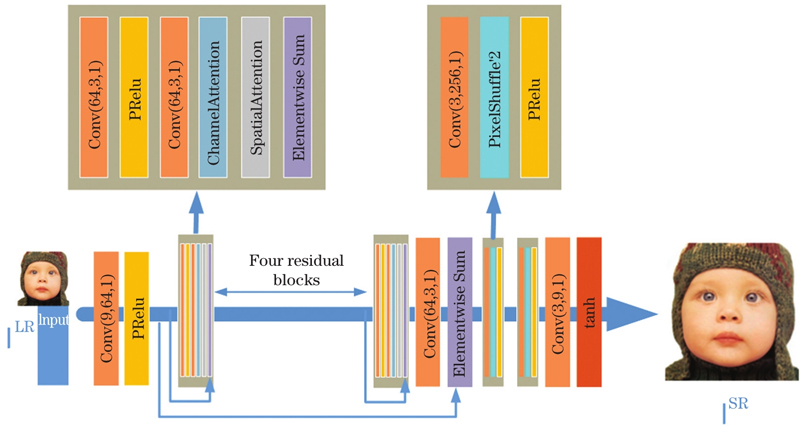
Fig. 1. Generator network structure
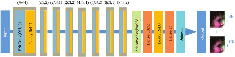
Fig. 2. Discriminator network structure
Fig. 3. Use of channel and spatial attention modules
Fig. 4. Reconstruction effects with different values of ε coefficient
Fig. 5. Comparison of residual blocks. (a)SRGAN; (b) proposed model
Fig. 6. Variation curve of generator function loss value
Fig. 7. Variation curve of discriminant function loss value
Fig. 8. Partial enlarged comparison diagrams of the “baby” reconstruction effect of five algorithms in Set5 test set
Fig. 9. Partial enlarged comparison diagrams of the “butterfly” reconstruction effect of five algorithms in Set5 test set
Fig. 10. Partial enlarged comparison diagrams of the “pepper” reconstruction effect of five algorithms in Set14 test set
Fig. 11. Partial enlarged comparison diagrams of the “fish” reconstruction effect of five algorithms in BSDS100 test set
Fig. 12. Partial enlarged comparison diagrams of the “room” reconstruction effect of five algorithms in Urban100 test set
Fig. 13. Partial enlarged comparison diagrams of the “baby” reconstruction effect in ablation experiment in Set5 test set
Fig. 14. Partial enlarged comparison diagrams of the “butterfly” reconstruction effect in ablation experiment in Set5 test set
Fig. 15. Partial enlarged comparison diagrams of the “lenna” reconstruction effect in ablation experiment in Set14 test set
|
Table 1. Comparison of PSNR values of various super-resolution reconstruction methods
|
Table 2. Comparison of SSIM values of various super-resolution reconstruction methods
|
Table 3. PSNR values of models with different module combinations on four test sets
|
Table 4. SSIM values of models with different module combinations on four test sets

Set citation alerts for the article
Please enter your email address
© Copyright 2018-2021 | Chinese Laser Press. All Rights Reserved 沪ICP备15018463号-20