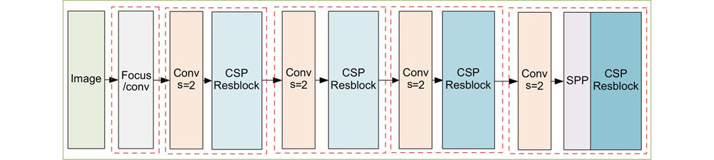
Fig. 1. YOLOv5 backbone network architecture diagram
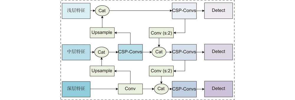
Fig. 2. Structure diagram of feature fusion module
Fig. 3. (a) Res-DConv module; (b) Receptive field mapping
Fig. 4. Improved module structure
Fig. 5. YOLOv5sm+ model architecture
Fig. 6. (a) Total number of category instances on the VisDrone dataset; (b) Classes confusion matrix of YOLOv5m algorithm
Fig. 7. The detection examples of different algorithms in the VisDrone UAV scene. (a) YOLOv5m model; (b) YOLOv5sm+ model; (c) YOLOv5s model
Fig. 8. Comparison of the detection effects of three algorithms in dense vehicle scenes. (a) YOLOv5m; (b) YOLOv5s; (c) YOLOv5sm+
Fig. 9. Detection comparison of improved algorithm in DIOR dataset. (a) YOLOv5s; (b) YOLOv5sm+
YOLOv5s | 感受野 | 通道 | YOLOv5sm | 感受野 | 通道 | Focus | 6 | 32 | Conv 3*3 (stride:2) | 3 | 24 | | | | Conv3*3 (dilation:2) | 15 | 48 | 下采样 | 10 | 64 | Conv3*3 (stride:2) | 19 | 96 | | | | Res-Block | 27 | 96 | C3_x1 | 18 | 64 | Res-Dconv | 51 | 96 | 下采样 | 26 | 128 | Conv 3*3 (stride:2) | 59 | 192 | C3_x3 | 74 | 128 | C3_x3 | 107 | 192 | 下采样 | 90 | 256 | Conv3*3 (stride:2) | 123 | 384 | C3_x3 | 186 | 256 | C3_x3 | 219 | 384 | 下采样 | 218 | 512 | Conv3*3 (stride:2) | 251 | 768 | Spp | 218~634 | 512 | Spp | 251~667 | 768 | C3_x1 | 282~698 | 512 | C3_x1 | 315~731 | 768 |
|
Table 1. Receptive field analysis table
下采样因子 | 3 | 4 | 5 | 最大感受野/pixel | 111 | 255 | 731 | 先验框范围 | 8*8~37*37 | 32*32~85*85 | 96*96~365*365 |
|
Table 2. Pre-setting anchors in response to the receptive field and down-sampling
目标种类 | Small (0×0~32×32) | Mid (32×32~96×96) | Large (96×96~) | 数量 | 44.44 | 18.63 | 1.704 |
|
Table 3. Statistics of different types of objects
深度 | 宽度 | mAP50 | mAP | BFLOPs | 0.33 | 0.5 | 0.502 | 0.288 | 16.5 | 0.33 | 0.75 | 0.540 | 0.319 | 36.3 | 1.33 | 0.5 | 0.525 | 0.311 | 35.4 |
|
Table 4. Performance comparison experiment results of depth and width models
Baseline | Res-Dconv | mAP50 | mAP | BFLOPs | √ | | 0.502 | 0.288 | 16.5 | √ | √ | 0.516 | 0.299 | 19.8 |
|
Table 5. Verification experiment results on Res-Dconv module
Baseline | SM | SCAM | SDCM | mAP | mAP50 | BFLOPs | Infer | AP-small | AP-medium | AP-large | 注:加粗字体为该列最优值。 | YOLOv5s | | | | 0.319 | 0.548 | 16.5 | 4.8 | 0.220 | 0.437 | 0.495 | | √ | | | 0.358 | 0.589 | 30.1 | 8.3 | 0.280 | 0.476 | 0.495 | √ | | √ | | 0.324 | 0.555 | 14.7 | 3.8 | 0.225 | 0.446 | 0.511 | √ | | | √ | 0.333 | 0.555 | 19.5 | 4.9 | 0.250 | 0.448 | 0.482 | | √ | | √ | 0.356 | 0.593 | 38.0 | 9.0 | 0.278 | 0.475 | 0.512 | | √ | √ | √ | 0.360 | 0.596 | 30.8 | 7.7 | 0.281 | 0.479 | 0.505 |
|
Table 6. The ablation experiment results of our algorithm modules on the VisDrone dataset
算法 | mAP50 | mAP | mAP75 | AP-small | AP-mid | AP-large | BFLOPs | Infer/ms | 注:+为添加改进模块的模型,*为多尺度测试结果,包含引用文献实验结果。 | YOLOv3 | 0.609 | 0.389 | 0.417 | 0.297 | 0.496 | 0.545 | 154.9 | 27.8 | Scaled-YOLOv4 | 0.620 | 0.400 | 0.428 | 0.305 | 0.514 | 0.626 | 119.4 | 27.1 | ClusDet[1] | 0.562 | 0.324 | 0.316 | - | - | - | - | - | HRDNet[1] | 0.620 | 0.3551 | 0.351 | - | - | - | - | - | YOLOv5s | 0.548 | 0.319 | 0.317 | 0.220 | 0.437 | 0.495 | 16.5 | 4.8 | YOLOv5m | 0.595 | 0.365 | 0.372 | 0.285 | 0.482 | 0.525 | 50.4 | 9.8 | YOLOX-s | 0.535 | 0.314 | 0.317 | 0.225 | 0.415 | 0.485 | 41.65 | 5.1 | MobileNetv3 | 0.554 | 0.329 | 0.329 | 0.245 | 0.443 | 0.495 | 23.8 | 8.0 | MobileViT | 0.555 | 0.333 | 0.337 | 0.249 | 0.442 | 0.418 | - | 13.7 | YOLOv5sm+ | 0.596 | 0.360 | 0.369 | 0.281 | 0.479 | 0.505 | 30.8 | 7.7 | YOLOv5sm+* | 0.606 | 0.367 | 0.378 | 0.295 | 0.478 | 0.439 | - | - |
|
Table 7. Detection performance of different algorithms on VisDrone dataset
模型 | BackBone | mAP50 | 注:加粗字体为该列最优值,包含其他文献对比结果。 | Faster R-CNN[33] | VGG16 | 0.541 | PANet[20] | ResNet50 | 0.638 | Retina-Net[24] | ResNet50 | 0.685 | 文献[32]
| ResNet50 | 0.732 | CAT-Net[34] | ResNet50 | 0.763 | YOLOv5sm+(ours) | - | 0.667 |
|
Table 8. Detection performance of different algorithms on DIOR dataset