On the design of high conversion efficiency quasi-optical mode converter for 140 GHz high-power gyrotron applications

Ming JIN; Dan-Yang WANG; Yi-Chi ZHANG; Yu-Nan HAN; Ming BAI

doi:10.11972/j.issn.1001-9014.2023.02.014

Abstract

A high conversion efficiency quasi-optical mode converter prototype is designed for 140 GHz TE_22,6 applications. The Denisov launcher is designed based on the periodic perturbation concept, leading to primary radiation field with low edge diffraction. Full-vector physical optics integration solver is used to model and analyze the 3-mirror system. And the 3-mirror iterative phase correction is applied based on the co-polarization field component, so as to achieve high-quality mode conversion. Specifically, the correction of the 1^st mirror sufficiently refines the non-ideal radiated fields from the launcher. It is then validated by numerical investigations that, comparing to the original quaritic mirrors, the phase-shaped mirror system leads to excellent conversion performance. The Gaussian content (η_v) of the output fields rises from 92.7% to 99.6%, while the power transmission efficiency (η_p) reaches 98.8%.

Keywords

high-power gyrotron output Gaussian content phase correction quasi-optical mode converter

Introduction

The quasi-optical mode converter（QOMC）is a vital device in the high-power Mega-Watt（MW）fusion heating gyrotron^［1-4］. It transforms the excited waveguide fields of TE_m，n mode which is not suitable for long-distance transmission，into the propagable fundamental Gaussian mode fields（FGMF）. For such an application，it is desired that the QOMC can be designed with a high conversion efficiency η_c，which includes the two aspects of output Gaussian content η_v and power efficiency η_p.

Modern QOMC generally consists of a Denisov launcher and the following multi-mirror system. In the Denisov launcher，periodic perturbations are applied on the inner circular wave-guide wall，to introduce mode coupling towards satellite modes，generating pre-focused Gaussian-like pattern at the launcher cut ^{［2，5-6］}. Comparing to classic Vlasov launcher，the Denisov launcher greatly reduces the edge diffraction at the launcher cut，and has become the foundation of high conversion performance QOMC ^{［3，7-9］}. The following mirror system generally comes with 3-5 mirrors，which build up a beam path keeping away from the electron beam while re-focusing and refining the beam profile ^{［2，10-14］}. The first mirror is generally for the necessary re-focusing of the horizontally diverging fields from the launcher，and the rest functions on refining the beam. For the mirror system，phase correction is a significant procedure in pursing high-conversion performance ^［14-15］.

Because the conversion-residual fields is diffusing and hard to control in space，pursing high conversion performance is a primary task in the QOMC design. In Ref.［10］，Jin，et al，reported the QOMC design with simulated η_v above 98%，In Ref.［13］，Liao，et al，reported high performance QOMC with simulated η_vof 99.8% based on 5 mirror phase correction. In Ref.［2］，it is concluded the performance of QOMC designs can be steadily at the level of 95%-97% in AIP（Institute of Applied Physics），Russian. Generally，more mirrors lead to more design freedoms in refining the output beam，but tend to increase the diffraction loss，possible thermal loss，system complexity and alignment difficulty. It is concluded the dissipation from the launcher is the source of diffraction loss across the multi-mirror reflection，hence effects are made towards optimized launcher designs ^{［12，17-18］}. And，reducing the number of the mirror while retaining good output quality is another path to reduce the diffraction loss ^［19］.

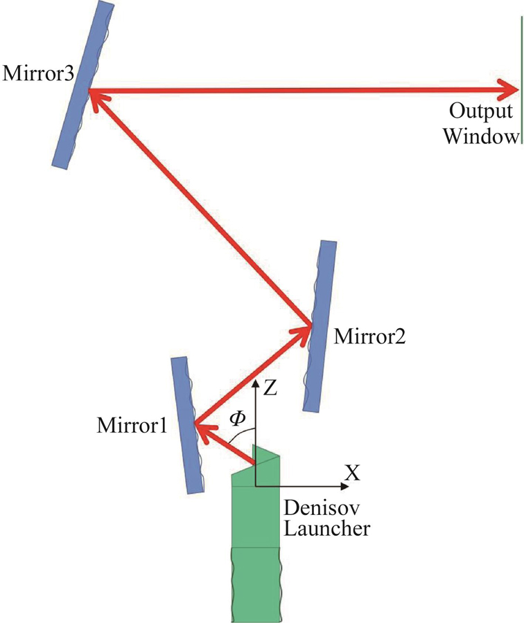
Figure 1.Configuration of 140 GHz TE_22，6 3-mirror quasi-optical mode converter

In a former work，a 3-Mirror 140 GHz TE₂₂₆ prototype was designed based on Denisov launcher and quadric mirrors，achieving output Gaussian content of 92.7% ^［9］. In this work，meticulous iterative phase correction is applied to the mirror system to pump up the output quality. It is shown in the numerical results，the optimized QOMC design achieves the excellent conversion performance in case of moderate number of mirrors：the Gaussian content reaches 99.62%，power efficiency reaches 98.76%，together they result in the total conversion efficiency of 98.38%. The reported mirror system optimization can be direct reference to high-performance QOMC design.

1　Optimization methodology on the mirror system

1.1　140 GHz TE_22,6 quasi-optical mode converter

The original 140 GHz TE_22，6 QOMC design starts from the Denisov launcher，then 3-quadric mirrors form the adjusting beam path ^［9］. The components layout configuration can be shown in Table 1. In the original design，the mirror 1 is derived based on geometric description of Vlasov launcher radiation，as a quasi-elliptical to horizontally re-converge the diffusing fields from the launcher. Then the mirrors 2 and 3 are designed based on parabolic and elliptical profiles，forming a focusing and refocusing beam path in the converter. The whole layout is presented in Fig. 2，in which the output beam pattern with the Gaussian content of 92.7% is also included. Further in Fig. 2，the focusing properties of each mirror are also concluded vertically and horizontally，along with the ray-tracing demonstration for the beam path in the converter.

Launcher Radius/mm	16.8	Launcher Radiation Angle/deg：	67.8
Launcher Height/mm	35.4	Center of Mirror 1（x，z，mm）	（-40，34.1）
Center of Mirror 2（x，z，mm）	（45，110）	Center of Mirror 3（x，z，mm）	（-130，320）
Center of Output Window（x，z，mm）	（234，320）	Waist Radius of Ref Gaussian Beam /mm	13.5

Table 1. Layout parameters of the 140 GHz TE_22,6 QOMC

View all Tables

Figure 2.Configuration of 140 GHz TE_22,6 3-mirror original quasi-optical mode converter, (a) vertical focusing functions of the mirrors in the original design (shown with ray-tracing), and the converted beam pattern at the output window, co-pol fields (E_y), normalized magnitude, linear, (b) horizontal focusing functions of the mirrors in the original design (shown with ray-tracing)

The main drawback of the original design，is that the quadric mirrors can not sufficiently correct the radiation fields from the Denisov launcher，in two aspects. First，the overall pattern of the launcher radiation is hard to be very close to Gaussian，then it is hard to adopt the non-ideal pattern of the launcher radiation into a excellent round-Gaussian pattern by using the quadric mirrors. Second，the radiation fields from the launcher contains edge diffraction and leakages，which are notable all along the beam path. As shown in Fig. 3，the non-ideal edge leakage can be observed in the surface current distribution on the Denisov launcher wall，marked as P1 and P2. Further，those signatures are notable in the illumination fields upon the first and last mirror，those actually become important restriction for an excellent field conversion.

Figure 3.Comparison of induced current distribution along the Denisov waveguide wall, and the illumination field distributions on the first and second mirror in the original QOMC design, for demonstrating the non-ideal edge fields，all the results are of normalized magnitude, in dB

1.2　Iterative mirror phase correction

It is desired the mirror system can correct the non-idealities in the launcher radiated fields. For this purpose the phase correction technique is an important solution. The 3-mirror system provides with sufficient freedom for the phase correction. For implementation，first，the radiation fields of the launcher by full wave simulation on a Huygens box，are utilized as the input of the phase correction from the source side. In this way，it is important that the edge effects are included in the launcher radiation. Similar works may consider the induced currents in the Brillouin region at launcher cut as the equivalent source ^{［11，14］}，that actually may leads to the omitting of the edge diffraction as an important factor for power leaking and beam pattern degradation.

Then，for the specific implementation of phase correction，a table of procedures can be concluded in Table 2，considering the whole 3-mirror iterative correction. For the necessary field propagation calculation procedure，full-vector physical optics（PO）integration（Eqs. 1-2）are utilized for calculating surface induced currents or fields for phase correction，so that the complex near-field propagation characteristics can be included in the simulation. And for the time-consuming PO integration，GPU-CUDA acceleration has been applied.

I Iteration 0

I.A Phase correction on the mirror 3（in detail）

（1） Forward calculation：

Ø Calculate the surface current（ ${\vec{J}}^{F_M 1} = 2 \hat{n} \times {\vec{H}}^{F_M 1}$ ）on the original Mirror 1 from the Huygens Box（ ${\vec{J}}^{H u y} = \hat{n} \times {\vec{H}}^{H u y}$ ， ${\vec{J}}_{M}^{H u y} = {\vec{E}}^{H u y} \times \hat{n}$ ），using Eq.（1）.

Ø Calculate the surface current（ ${\vec{J}}^{F_M 2} = 2 \hat{n} \times {\vec{H}}^{F_M 2}$ ）on the original Mirror 2 from the Mirror 1 surface current（ ${\vec{J}}^{F_M 1}$ ），using Eq. 1.

Ø Calculate the illumination fields（ ${\vec{E}}^{F_M 3}$ ）on the Mirror 3 correction lattice，from the Mirror 2 surface current（ ${\vec{J}}^{F_M 2}$ ），using Eq. 2.

（2） Backward calculation：

Ø Calculate the referencing fields（ ${\vec{E}}^{B_M 3}$ ）on the Mirror 3 correction lattice，from the referencing fundamental Gaussian field sources（ ${\vec{J}}_{M}^{G} = 2 {\vec{E}}^{G} \times \hat{n}$ ），using Eq. 2.

（3）Phase Correction：

Ø Take the co-polar component of forward fields（ $E_{y}^{F_M 3}$ ）and backward fields（ $E_{y}^{B_M 3}$ ）on Mirror 3 correction lattice，turns the phase difference into geometry correction，using Eqs. 3-4. Specifically，the diagram of phase correction can be concluded in Fig. 4. After the phase correction process，the generated mirror is described as triangle meshes which can be exported as a STL format file for further calculation and fabrication.

II Iteration 1..N

II.A Phase correction on the mirror 2（in detail）

（1） Forward calculation：

Ø Calculate the surface current（ ${\vec{J}}^{F_M 1} = 2 \hat{n} \times {\vec{H}}^{F_M 1}$ ）on the Mirror 1 from the Huygens Box（ ${\vec{J}}^{H u y} = \hat{n} \times {\vec{H}}^{H u y}$ ， ${\vec{J}}_{M}^{H u y} = {\vec{E}}^{H u y} \times \hat{n}$ ），using Eq. 1.

Ø Calculate the illumination fields（ ${\vec{E}}^{F_M 2}$ ）on the Mirror 2 correction lattice，from the Mirror 1 surface current（ ${\vec{J}}^{F_M 1}$ ），using Eq. 2.

（2） Backward calculation：

Ø Calculate the surface currents（ ${\vec{J}}^{B_M 3} = 2 \hat{n} \times {\vec{H}}^{B_M 3}$ ）on the Mirror 3，from the referencing fundamental Gaussian pattern（ ${\vec{J}}_{M}^{G} = 2 {\vec{E}}^{G} \times \hat{n}$ ），using Eq. 1.

Ø Calculate the referencing fields（ ${\vec{E}}^{B_M 2}$ ）on the Mirror 2 correction lattice，from the Mirror 3 surface current（ ${\vec{J}}^{B_M 3}$ ），using Eq. 2.

（3） Phase correction..

II.B Phase correction on the mirror 1（in detail）

（1） Forward calculation：

Ø Calculate the illumination fields（ ${\vec{E}}^{F_M 1}$ ）on the Mirror 1 from the Huygens Box（ ${\vec{J}}^{H u y} = \hat{n} \times {\vec{H}}^{H u y}$ ， ${\vec{J}}_{M}^{H u y} = {\vec{E}}^{H u y} \times \hat{n}$ ），using Eq. 2.

（2） Backward calculation：

Ø Calculate the surface current（ ${\vec{J}}^{B_M 2} = 2 \hat{n} \times {\vec{H}}^{B_M 2}$ ）on the Mirror 2 from the Mirror 3 surface current（ ${\vec{J}}^{B_M 3}$ ），using Eq. 1.

Ø Calculate the referencing fields（ ${\vec{E}}^{B_M 1}$ ）on the Mirror 1 correction lattice，from the Mirror 2 surface current（ ${\vec{J}}^{B_M 1}$ ），using Eq. 2.

（3） Phase correction..

II.C Phase correction on the mirror 2..

II.D Phase correction on the mirror 3..

Table 2. Procedures of iterative multi-mirror phase correction

View all Tables

\begin{array}{l} \vec{H} (\vec{r}) = \frac{1}{j ω μ} [\frac{(3 - {k_{0}}^{2} R^{2} + j 3 k_{0} R) (\vec{R} \times (\vec{R} \times {\vec{J}}_{M} ({\vec{r}}^{'})))}{4 π R^{5}} + \\ \frac{2 (j k_{0} R + 1)}{4 π R^{3}} \cdot {\vec{J}}_{M} ({\vec{r}}^{'}))] e^{- j k_{0} R} d s^{'} - \\ \int_{S} \frac{(- j k_{0} R - 1) (\vec{R} \times \vec{J} ({\vec{r}}^{'}))}{4 π R^{3}} e^{- j k_{0} R} d s^{'} \end{array}

，（1）

here，Eq. 1 can be utilized to calculate the induced surface currents on each mirror（ $\vec{J} = 2 \hat{n} \times \vec{H}$ ）.

\begin{array}{l} \vec{E} (\vec{r}) = \frac{1}{j ω ε} [\frac{(3 - {k_{0}}^{2} R^{2} + j 3 k_{0} R) (\vec{R} \times (\vec{R} \times \vec{J} ({\vec{r}}^{'})))}{4 π R^{5}} + \\ \frac{2 (j k_{0} R + 1)}{4 π R^{3}} \cdot \vec{J} ({\vec{r}}^{'}))] e^{- j k_{0} R} d s^{'} - \int_{S} \frac{(- j k_{0} R - 1) (\vec{R} \times {\vec{J}}_{M} ({\vec{r}}^{'}))}{4 π R^{3}} e^{- j k_{0} R} d s^{'} \end{array}

，（2）

where k₀ is the free-space wave-number，and $\vec{R} = \vec{r} - {\vec{r}}^{'}, R = |\vec{R}|$ . Here，Eq. 2 can be utilized to calculate the radiated E-fields at output window or at mirror lattices for phase correction.

Δ p h a s e (\vec{r}) = a r g ({E_{y}^{B}}^{*} (\vec{r}) / E_{y}^{F} (\vec{r}))

，（3）

\begin{array}{l} Δ h (\vec{r}) = \frac{Δ p h a s e (\vec{r})}{2 \cdot k_{0} c o s θ (\vec{r})}, c o s θ (\vec{r}) = {\hat{k}}_{i} \cdot \hat{n} (\vec{r}), {\vec{r}}^{C o r r e c t e d} \\ = {\vec{r}}^{o r i} + Δ h ({\vec{r}}^{o r i}) \hat{n} ({\vec{r}}^{o r i}) \end{array}

，（4）

here， $\hat{n} (\vec{r})$ is normal direction at the local mirror surface，and ${\hat{k}}_{i}$ stands for the incident direction of the illumination beam. And Eq.（3）and（4）are for generating local position shifts in the phase correction process.

Besides the numerical implementation of iterative phase correction，it is further important to discuss the field conversion performance in the view of field characteristics. In this work，for the typical 3-Mirror TE_22，6QOMC，both the 2-mirror（including M2 and M3），and 3-mirror（including M1，M2 and M3）phase correction processes，are separately and comparatively excised. The results will be analyzed in next section.

2　Results and discussions

In this section，the results of the optimized QOMC are to be analyzed. Specifically，for the 2-mirror phase correction considering Mirror 2 and Mirror 3，as well as 3-mirror phase correction，10 times of iterative phase correction are implemented，as demonstrated in last section. In Fig. 4，the corresponding results of Gaussian content in the output fields are plotted（the Gaussian content is defined in Eq.（5））. Specifically，in the case of 3-mirror phase correction，the illumination field patterns on each mirror and output fields are plotted in Fig. 5，after different round of iterative phase correction. The gradually improved illumination conditions especially on the Mirror 3 during the iterative correction can be clearly observed，which leads to the refined output field pattern. That means the iterative process works properly. It is also important that the non-ideal edge fields sourced from the launcher（Fig. 3）can be reformed in the 3-mirror correction process.

η_{v} = |\frac{\iint {\vec{E}}_{t} \cdot {\vec{G}}_{t}^{*} d s \cdot \iint {\vec{E}}_{t}^{*} \cdot {\vec{G}}_{t} d s}{\iint {\vec{E}}_{t} \cdot {\vec{E}}_{t}^{*} d s \cdot \iint {\vec{G}}_{t} \cdot {\vec{G}}_{t}^{*} d s}|

，（5）

Figure 4.Diagram of phase correction mirror generation，based on Eq.（3）and Eq.（4）

Figure 5.Computed Gaussian contents in the output field at output window，after each round of phase correction

where ${\vec{E}}_{t}$ stands for tangential fields on the output aperture，and ${\vec{G}}_{t}$ is the pure E_y polarized Gaussian Fields.

At the same time，as presented in Fig. 5，the 3-mirror phase correction leads to excellent high-η_v performance，which is clearly better than the 2-mirror phase corrected results. Further in Fig. 7，the converted E-fields on the output window are presented. As can be observed，the 3-mirror corrected results show better Gaussian-like pattern（magnitude）and larger phase-flatten phase area，over the 2-mirror corrected results. Actually，that the pair of 2-mirror already form a sufficient beam shaping link，and from view of practical application，less phase correction mirrors lead to less fabrication and assemble difficulties. Therefore，it is interesting and of information to lucubrate the reason why 3-mirror phase correction performs notably better.

Figure 6.Illumination field patterns on each mirror，and output fields（Ey，normalized magnitude，dB），after different rounds of iterative 3-mirror phase correction，the field results are calculated by Eq.（1）and（2）

Figure 7.Converted fields at output window in both cases of 2-mirror corrected converter and 3-mirror corrected converter. The referencing Gaussian beam is with beam waist of ω₀ = 13.5 mm at the output window

Specifically，comparing within the cases of original mirrors，2-mirror corrected mirrors，and 3-mirror corrected mirrors the illumination fields on the reflecting mirrors are plotted in Fig. 6，to reveal the beam shaping mechanism in the phase correction process.

Firstly，in the original quadric mirror systems（Fig. 8（a）），the non-ideal edge fields are observed in the illuminating fields on all the mirrors，that means the edge effects sourced from launcher radiator are not corrected in the quadric mirror systems. Actually，the edge fields are dividing from the main beam along the beam path. That is because the edge diffraction in launcher radiation acts differently from the main beam，therefore it doesn’t concentrate along the beam path designed based on the main beam characteristics.

Figure 8.Illumination Field patterns（E_y，normalized magnitude，dB）on each mirror，in cases of original quadric mirror systems，2-mirror corrected mirror system，and 3-mirror corrected mirror system. The illuminated field results are calculated by Eqs.（1）and（2）

Secondly，consider the 2-mirror corrected results，the illumination fields on the last mirror is notably corrected towards a round Gaussian，leading to good output quality as shown in Fig. 8（b），thanks to the phase correction on the mirror 2. However，it is important in the illumination fields onto mirror 2 that the edge fields are already divided from the main beam area，which clearly brings difficulties in the beam shaping. As shown in Fig. 8（b），non-ideal edge fields are suppressed but still existing in the illumination fields on mirror 3.

Thirdly and comparatively，in the 3-mirror correction，the first mirror correction is included，which offers the ability to re-focus the edge diffracted fields back into the main beam，as an improved illumination condition for following mirrors. It is important that the edge fields can be corrected by the first mirror before they become more departed from the main beam during the propagation. Consequently，the illumination fields on Mirror 3 further approach to the ideal round Gaussian pattern，resulting in the excellent output beam quality（Fig. 8（c））.

From this set of comparison and analysis，it can be concluded that：the phase correction on the first mirror is important，as it offers the possibility to correct the launcher edge diffraction in an early stage，leading to good illumination condition for following mirrors in achieving excellent output beam quality.

Finally，the overall performance of 3-mirror corrected QOMC is to be demonstrated. In Fig. 9，the corrected mirrors and output fields at different apertures are presented. It is important that，the power efficiency of the optimized converting mirrors is also good：η_p= P_output / P_in= 98.76%，which is defined as the ratio of output fields power to the radiating power from the launcher. The resulted overall conversion efficiency η_c_{=_{η_pη_v}}，achieves 98.38%. Actually，the iterative phase correction tends to converge the diffusing fields back into the main beam path，hence is also helpful in improving the power efficiency. Specifically，the η_prises from 98.29%（after iteration 0）to 98.76%（after iteration 10）during the 3-mirror iterative phase correction. It should be noted，the simulated η_p discussed in this paper does not include the factor of mirror thermal loss.

Figure 9.Showcase of output fields at different apertures，of the 3-Mirror corrected TE₂₂₆ QOMC design（a）：concluded total conversion efficiency η_c，Gaussian content η_v and power efficiency η_p of the aperture fields distant from the output window，（b）：output field patterns at different apertures，co-pol fields（E_y），normalized magnitude，linear

Also，as can be observed in Fig. 9，the high quality Gaussian-like output beam can maintain round Gaussian pattern all along the propagation path. As concluded in Fig. 9（a），as the beam propagates away from the output window，the Gaussian content η_v of the aperture fields gets slightly larger（referencing to the Gaussian beam with beam waist ω₀ = 13.5 mm at the output window），while the power efficiency η_p gets slightly smaller，maintaining a good total conversion efficiency η_c along the beam path. That further demonstrates the high-quality of the transformed output fields.

3　Conclusions

In summary，we report the optimization design on the 140 GHz TE_22，6 QOMC. For the 3-mirror system results，the optimized QOMC achieves excellent performance of output Gaussian content of 99.62%，power efficiency of 98.76%，and total conversion efficiency of 98.38%，based on the mirror system with moderate complexity. In the beam shaping investigation，importance of first mirror correction is concluded. The first mirror correction offers the possibility to correct the diffusing edge diffraction from launcher at the early-stage，leading to good illumination condition for following beam shaping procedures，which is important in pursing excellent output field quality. The design methodology for high-performance QOMC presented in this work can offer direct reference to the related fields. As an outlook，it would be much more meaningful if the high conversion performance can be retained in actual fabricated prototypes，following work will be focused on further refining the design methodology to meet the challenges from manufacturing and testing.

References

[1] G Nusinovich, M Thumm, M Petelin. The Gyrotron at 50: Historical Overview. J. Infrared Millim. Terahertz Waves, 35, 325-381(2014).

[2] A Litvak, G Denisov, M Glyavin. Russian gyrotron: Achievements and trends. IEEE Journal of Microwaves, 1, 260-268(2021).

[3] J Jin. Quasi-optical mode converter for a coaxial cavity gyrotron, 46-48(2007).

[4] Y Zhang, Xu Zeng, M Bai et al. The development of 170 GHz, 1MW gyrotron for fusion application. Electronics, 11, 1279(2022).

[5] A Bogdashov, G Denisov. Asymptotic theory of high-efficiency converters of higher-order waveguide modes into eigenwaves of open mirror lines. Radiophys. Quantum Electron, 47, 283-296(2004).

[6] G Denisov, A Kuftin, V Malygin et al. 110 GHz gyrotron with a built-in high-efficiency converter. Int J. electronics, 72, 1079-1091(1992).

[7] M Thumm, X Yang, A Arnold et al. A high-efficiency quasi-optical mode converter for a 140-GHz 1MW CW gyrotron. IEEE Trans. Electron Devices, 52, 818-824(2005).

[8] W Wang, D Liu, S Qiao et al. Study on terahertz denisov quasi-optical mode converter. IEEE Trans. Plasma Sci., 42, 346-349(2014).

[9] D Xia, M Jin, M Bai. Asymmetrical mirror optimization for a 140 GHz TE22,6 quasi-optical mode converter system. Chin. Phys. B., 26, 074101(2017).

[10] J Jin, B Piosczyk, M Thumm et al. Quasi-optical mode converter/mirror system for a high-power coaxial -cavity gyrotron. IEEE Trans. Plasma Sci., 34, 1508-1515(2006).

[11] G Zhao, Q Xue, Y Wang et al. Design of quasi-optical mode converter for 170-ghz TE32,9-mode high-power gyrotron. IEEE Trans. Plasma Sci., 47, 2582-2589(2019).

[12] Q Huang, L Hu, G Ma. Quasi-optical mode converter for a high power TE8,3-mode gyrotron. AIP Advances, 12, 075116(2022).

[13] S Liao, R Vernon. Sub-THz beam-shaping mirror system designs for quasi-optical mode converters in high-power gyrotrons. J. Electromagn. Wavs and Appl., 21, 425-439(2007).

[14] S Xu, J Yang, H Wang et al. Design of a quasi-optical mode converter for a 170 GHz gyrotron. J. Infrared Milli. Waves, 41, 557-562(2021).

[15] B Katsenelenbaum, V Semenov. Synthesis of phase corrector shaping a specified field. Radio Eng. Electron. Phys, 12, 223-231(1967).

[16] J Liu, J Jin, M Thumm et al. Vector method for synthetic of adapted phase-correcting mirrors for gyrotron output couplers. IEEE Trans. Plasma Sci., 41, 2489-2495(2013).

[17] J Jin, J Flamm, J Jelonnek et al. High-efficiency quasi-optical mode converter for a 1-MW TE32,9-mode gyrotron. IEEE Trans Plasma Sci., 41, 2748-2753(2013).

[18] J Jin, M Thumm, G Gantenbein et al. A numerical synthesis method for hybrid-type high-power gyrotron launchers. IEEE Trans Microwave Theory Tech., 65, 699-706(2017).

[19] M Jin, X Li, D Xia et al. A compact dual-mirror design of quasi-optical mode converter for gyrotron application. IEEE Antennas Wireless Propagat. Lett., 21, 1032-1036(2022).