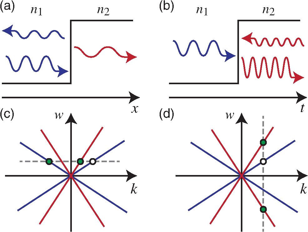
Fig. 1. Scattering at (a) a spatial discontinuity, generating transmitted and reflected waves propagating in different media with refractive indices n1 and n2, and (b) a temporal discontinuity, generating forward and backward waves propagating in the same medium. (c), (d) Illustration of the respective scattering processes on a dispersion diagram: the blue and red lines denote the dispersion cone for the two media. Note how the frequency ω is conserved in a spatial scattering process, and coupling occurs to forward and backward modes in the two different media, whereas in a time-scattering process the momentum k is conserved, and the two scattered waves are both embedded in the new medium.

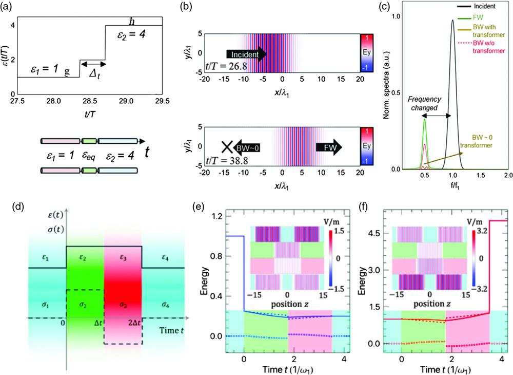
Fig. 2. (a) Schematic of the antireflection temporal coatings proposed in Ref. 39. (b) Numerical results for the field distribution before and after the temporal scattering, showing the incident and transmitted waves, with minimized reflection due to the temporal coating shown in (a). (c) Spectra of the incident, forward, and backward waves. (d) Schematic of TPT symmetric structures proposed in Ref. 40. (e) and (f) The time evolution of the normalized energy (solid curves) and its two constitutions (circle symbols for interferences and the dashed curves for another). (e) Maximum total power and (f) minimum total power. Insets are the field distributions in simulations before, during, and after the TPT slabs. Figures adapted from Refs. 39 and 40.

Fig. 3. (a) A conventional prism decomposing white light into its frequency components in different directions. (b) An inverse prism that maps the light with different momentum into different frequencies. (c) Implementation of the inverse prism proposed in Ref. 28. (d) Temporal aiming proposed in Ref. 43. (e) The conventional Brewster angle. (f) Temporal Brewster angle described in Ref. 44. Figures adapted with permission from Refs. 28, 43, and 44.

Fig. 4. (a) Temporal reflection of graphene plasmons reported in Ref. 54. (b) Impedance matching using a time-switched transmission line.⁵⁶ (c) Time-switched thin absorber in Ref. 57. (d) Unitary excitation transfer between two coupled circuit resonators.⁵⁸ (e) Temporal deflection caused by isotropic-to-anisotropic switching on meta-atoms.⁵⁹ (f) Temporal switching of structural dispersion for ultrafast frequency-shifts, proposed in Ref. 60. (g) Corresponding frequency spectra for the switching in (f). Figures adapted from Refs. 54, 56, 57, 58, 59, and 60.

Fig. 5. (a), (b) Example of a (finite) layered (a) PSC and (b) PTC, and corresponding wave behaviour within the respective band gaps. (c) Band structure of a PTC, showing k-gaps and Zak numbers of the different bands. (d) Change of Zak phase across the first k-gap. (e) Example of an edge between two PTCs with opposite Zak phase. (f) Numerical demonstration of the effect of a temporal edge between two topologically inequivalent PTCs: the parametric amplification process is interrupted and the wave amplitude is depleted for a few periods following the temporal edge, forming a temporally localized state. Figures adapted from Ref. 72.

Fig. 6. (a) The resonant modes of a structure form a lattice in the frequency dimension. (b) Hopping through its sites can be enabled by time modulation, which can couple their different frequencies. (c) The resulting Hamiltonian is analogous to that of electrons in a periodic ionic potential. (d) A ring resonator combined with a modulator can reproduce such a model, (e) enabling hopping between its equally spaced resonant modes.⁷⁷ (f)–(h) A synthetic dimension may be constructed in a tight-binding model by introducing long-term coupling between the elements of a chain. In the time-domain, this can be realized by modulating the system at multiple frequencies.⁷⁸ (i), (j) A spatially 1D chain of ring resonators can be combined with temporal modulation to form a synthetic 2D lattice.⁷⁹ Figures adapted from Refs. 77–79" target="_self" style="display: inline;">–79.

Fig. 7. (a) Two resonators coupled via a combination of constant (k0), time-dependent Hermitian (Δk′), and time-dependent non-Hermitian (Δk′′) coupling terms. (b)–(e) Wave amplitude under excitation via port 1 in the two resonators (orange and blue) for two arbitrary values of Δk′ at the excitation frequency (ω1) and the two sidebands for (b) k0≠0 and Δk′′=0 (energy stored in both sidebands and both resonators); (c) Δk′′=0 and k0=0 (energy channeled to sideband frequencies is all in the second resonator while the first only hosts the input frequency); (d) Δk′=Δk′′ and k0≠0 (energy gained is nonreciprocally channeled into the upper sideband and it is distributed over both resonators); (e) Δk′=Δk′′ and k0=0 (energy gained is nonreciprocally channeled only into the upper sideband and uniquely in the second resonator).⁸⁶ (f) A random sequence of temporal δ-kicks results in (g) universal statistics observed by the energy in the system U. The energy at the N’th kick UN is plotted against the step number N.⁸⁷ Figures adapted from Refs. 86 and 87.

Fig. 8. (a) Light scattered from a flat, time-varying metasurface can access a locus of states that form a hyperbola in phase space, as opposed to an ellipse in spatial metasurfaces. (b) Implementation of a time-modulated metasurface at GHz frequencies. (c) A 1-MHz modulation performs efficient frequency conversion through time-modulation.¹⁰² (d) Illustration of surface-wave excitation via the Wood anomalies using (e) spatial and (f) temporal modulation of (g) a surface. (h) Example of the Wood anomaly observed in transmission, the surface-wave excitation is explicitly shown in (i) from a finite-element-time-domain simulation.¹⁰¹ Figures adapted from Refs. 102 and 101.

Fig. 9. (a) Space–time diagram of a space–time crystal with alternating refractive indices ni and nj, spatiotemporal lattice vector p and velocity vm. (b) Double-period space–time crystal, characterized by two different lattice vectors pA and pB, and two different velocities vm1 and vm2.¹¹⁹ (c) The band structure for a spatial crystal with ε∼cos(gz−Ωt) becomes asymmetric as (d) a finite temporal component Ω, and therefore a finite modulation velocity vm=Ω/g, are introduced. This is caused by reciprocal lattice vectors (dashed arrows) acquiring a non-zero frequency component. The angle formed by the reciprocal lattice vectors with the slope of the bands determines [(c), (d)] a subluminal and [(e), (f)] a superluminal regime.¹²⁰ (g) Nonreciprocal mode-coupling in a space–time-modulated waveguide: the modulation can couple forward modes between them as their frequencies and momenta are matched by the space-time modulation, while two backward waves are not coupled, so that an impinging backward wave is effectively unchanged.¹²¹ Figures adapted from Refs. 119, 120, and 121.

Fig. 10. (a)–(c) Angular momentum biasing: a directional modulation along a ring resonator splits the degeneracy between clockwise and anticlockwise traveling states (a),¹³⁸ in analogy with the Zeeman splitting of electronic states in a magnetic field (b),¹³⁸ this can be realized by discretizing the elements of the ring, e.g., periodically modulating three strongly coupled resonators, with a phase of 120 deg between them (c).¹³⁹ (d) Example of operation of a nonreciprocal ring resonator coupled to two waveguides: excitation from the bottom (top) of the channel waveguide (on the right of the ring) excites a counterclockwise (clockwise) mode, whose resonant frequency has been offset from the one of the clockwise (counterclockwise) mode, so (e) the direction of excitation determines the efficiency of the coupling to the resonator, and hence of the transmission to the output port of the channel waveguide.¹³⁸ (f), (g) Theoretical and (h) experimental performance of an RF circulator made with angular-momentum biased resonators: (f) and (g) the reciprocal response in the absence (f) and presence (g) of angular biasing, and (h) the performance of the experimental implementation of the circulator.¹³⁹ Figures adapted from Refs. 138 and 139.

Fig. 11. (a)–(c) A synthetic space–time-modulated crystal (a) is formally equivalent to a fictitious moving bianisotropic time-invariant crystal (b) when vm<c0. The velocity of the equivalent moving crystal is identical to the modulation speed vm; in the long-wavelength limit, the system response can be homogenized (c) and the crystal behaves as a uniaxial dielectric moving with speed vD. The sign of vD is not necessarily coincident with the sign of v. (d) Dispersion of waves in the effective medium as shown in (c). When only one of the material parameters is spatiotemporally modulated, the dispersion is symmetric, and the equivalent drag velocity vanishes (blue lines). However, when both ε and μ are modulated, the dispersion is asymmetric (red lines, assuming vD>0). The waves that propagate in the direction of vD have a larger group velocity than the waves that propagate in the opposite direction.¹⁶¹ (e) Drag velocity vD and (f) effective bianisotropic coefficient ξef as a function of the modulation speed vm for a representative space–time-modulated crystal: the velocity of the equivalent moving medium and the magnetoelectric coupling coefficient flip sign in the transition from the subluminal to the superluminal regime. The luminal regime is marked as a shaded area in (e) and (f). Figures adapted from Ref. 163.

Fig. 12. (a) Time dependence of the electric field intensity at the output port transmitted through different thicknesses (blue to red) d of luminal crystal. (b) In the gain region, the permittivity gradient is positive, and vice versa. The gain is maximum at the points (in time or space) where the velocity of the waves matches the velocity of the grating. (c), (d) Power spectra of the transmitted waves (c) for input frequency ω0=8Ω, with Ω the modulation frequency, and (d) for a DC input field (ω0=0), showing the frequency generation responsible for the overall gain.^120,177 (e), (f) Trajectories of a point of constant phase along the spacetime variable X=x−vmt: (e) outside of the localization regime (resulting in oscillations that periodically compress and decompress the pulse) and (f) within the localization regime, resulting in the amplification and compression described in (a)–(d).¹⁷⁶ Figures adapted from Refs. 120, 176, and 177.

Fig. 13. Examples of applications of space–time metasurfaces. (a) An isolator based on the unidirectional excitation of evanescent modes. (b) Waves scattering off an STM experience a nonreciprocal phase shift. (c) An STM-based circulator.¹⁰⁴ (d) Illustration of an experimentally realized space–time coding metasurface, consisting of a square array of individual voltage-controlled elements with binary impedance values, enabling encoding and imprinting of arbitrary phase and amplitude modulation onto different scattered harmonics for (e) beam-steering and shaping.¹¹⁴ (f) Illustration of wave power combining using STMs: incoming waves with frequency ω0 coming from a discrete range of different angles can be scattered toward the same outgoing direction by imprinting the necessary frequency-wavevector shifts via the STM.¹⁰⁸ (g) A proposal of an angular momentum-biased metasurface for the generation of orbital angular momentum states: each azimuthal section is temporally modulated with a different relative phase, imparting the necessary angular-momentum bias. Figures adapted from Refs. 104, 108, 114, and 181.

Fig. 14. (a), (b) Concept of photocarrier excitation and time-refraction in ITO:²¹⁵ (a) A pump pulse transfers energy to the electrons in the conduction band, leading to a temporal variation in the refractive index. (b) As the probe experiences different indices at different delays, its spectral content will be shifted (redshift for negative delay, blueshift for positive). (c)–(f) Measured time-refraction, phase conjugation, and negative refraction signals from a 500-nm-thick AZO slab pumped by 105 fs pulses, at an energy of 770GW/cm2 in a degenerate pump-probe experiment at 1400 nm.²¹⁶ (g) Strong coupling between a plasmonic antenna and an ENZ thin film:²¹⁷ electric field |E|2 distribution obtained from FDTD for an ITO layer thickness of 40 nm and Au antenna length of 400 nm. (h) Resulting field distribution as a function of depth.²¹⁷ (i)–(k) Probe spectrum at various delays for a central wavelength of 1304 nm for 50 fs pulses in a strongly-coupled plasmonic antenna-ENZ system.²¹⁸ The increase in modulating pump intensities (0.5, 1, and 2GW/cm2) leads to a shift near zero delay. Figures adapted from Refs. 216 to 218.

Fig. 15. (a) Schematic of a Si metasurface engineered to support collective high-Q Fano resonances.²³⁵ (b) Schematic of the self-induced blueshift of harmonics in the resulting Si nanoantenna cavity:²³⁵ photons in the antenna will undergo a blueshift due to the rapidly changing permittivity of the medium before being upconverted via third-harmonic generation. (c) Measured spectral evolution for an 80-fs pump pulse length in a GaAs high-Q metasurface.²³⁶ The fringes are measured on only one side of the spectrum due to the breaking of time-reversal symmetry caused by the modulation. (d) Schematic of a nonreciprocal Si metasurface:²³⁷ the traveling wave modulation breaks the space–time symmetry of the reflection phase change. Figures adapted from Refs. 235 to 237.