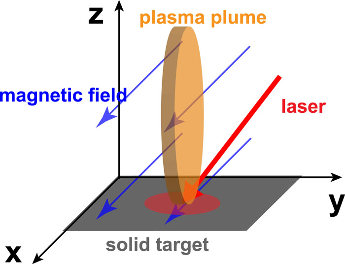
Fig. 1. Schematic of the simulation setup. The solid target is in the xy plane, the direction of the externally applied magnetic field is along the x axis, and the plasma plume expands along the z axis.

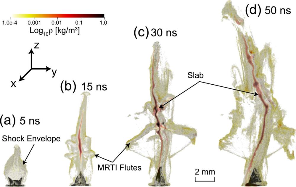
Fig. 2. Plasma dynamics and slab formation. (a)–(d) show global 3D renderings of the decimal logarithm of the mass density at different times (5, 15, 30, and 50 ns) after the laser pulse.

Fig. 3. Decimal logarithm of the mass density ρ (A) and temperatures T_e (B) and T_i (C) of the plasma plume sliced in the middle of the xz plane (a) and the yz plane (b) at different times 8, 18, 28, 38, and 48 ns (1–5). The temperatures in (B) and (C) share the same color map. The magnetic field directions are shown in (A1a) and (A1b).

Fig. 4. Plasma expansion and diamagnetic cavity formation: decimal logarithm of the electron number density integrated along or perpendicular to the magnetic field, i.e., the xz plane (a) or the yz plane (b), at 5 ns after the laser ablation. The color map corresponds to log₁₀∫n_edy in (a) and log₁₀∫n_edx in (b), in cm⁻². The black arrows show the direction and magnitude of the velocities, and the light blue lines and arrows show the direction of the magnetic field in the xz plane (they do not appear as continuous lines, because they are taken out of the sliced plane).

Fig. 5. MRTI growth during slab formation. (a) Zoomed view of the plasma/vacuum interface at t = 8 ns. Since the density map here is a slice at the middle plane x = 0, the color map corresponds to log₁₀ n_e in cm⁻³. Cyan lines show the contours of the current density magnitude, while the dashed line contours show the ion temperature T_i. (b) Temperature dependence of the fastest growing mode and the growth time for MRTI.

Fig. 6. Slab formation. (a) Collapse of the cavity at t = 15 ns around 3 mm < z < 5 mm (highlighted by the gray box). (b) Fully grown flutes at t = 30 ns reach the boundary of y = 4 mm. The collapsed region propagates along the z direction, arriving at 5 mm < z < 8 mm, and the slab is formed. The color map corresponds to log₁₀∫n_edx in cm⁻². The black arrows are the velocity vectors.

Fig. 7. Slab propagation with different initial magnetic field strengths in the simulation with asymmetric perturbation. (a)–(c) are for B_x0 = 10, 20, and 30 T, respectively. The color map corresponds to log₁₀∫n_edx in cm⁻².

Fig. 8. Typical spatial pattern of the laser intensity deposition on target in related experiments. The pattern is due to the fact that the laser is actually defocused on the plane of the target, so that its intensity is not too large, and hence we have on target a laser pattern with diffraction rings, which is typical of an intermediate plane before focus. The color map represents the normalized intensity.

Fig. 9. Spatial distribution of the Bessel-like perturbation of the plasma velocity: (a) u_1,1, for the m = 1, n = 1 mode; (b) u_1,2, for the m = 1, n = 2 mode. Other parameters are r₀ = 0.5 mm, α_1,1 = 3.8317, and α_1,2 = 7.0156. The color map corresponds to the perturbation strength.

Fig. 10. Slab propagation with different modes of Bessel-like perturbation for different magnetic field strengths at the end of the simulation at t = 50 ns. The color map corresponds to log₁₀∫n_edx in cm⁻², i.e., to the decimal logarithm of the electron number density integrated along the external magnetic field. (a) and (b) are for B_x = 10 T, while (c) and (d) are for B_x = 30 T. In (a) and (c), the initial Bessel-like perturbation is in the m = 1, n = 1 mode, while in (b) and (d), it is in the m = 1, n = 2 mode.

Table 1. Measured plasma conditions and calculated dimensionless parameters for the case with initial magnetic field B_x0 = 30 T in different regions as indicated in Fig. 2, i.e., the shock envelope at t = 5 ns, the MRTI flutes at t = 30 ns, and the slab at t = 50 ns. λ_mfp,s (with s = i and e for ions and electrons, respectively) is the mean free path³⁹ and r_L,s is the Larmor radius. The Mach number is the ratio of the flow velocity to the sound velocity, while the Alfvénic Mach number is the ratio of the flow velocity to the Alfvén velocity. The thermal and dynamic beta parameters are the ratios of the plasma thermal and ram pressures, respectively, to the magnetic pressure.