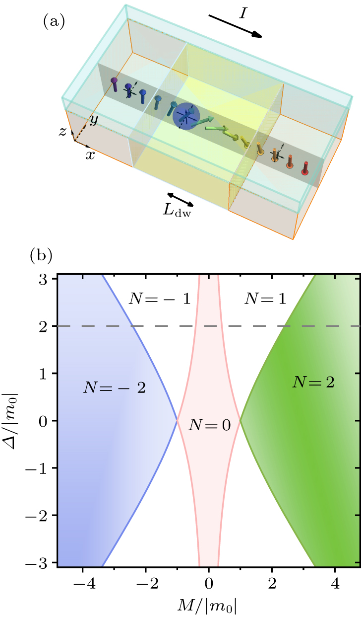
Fig. 1. (a) Schematic diagram for the QAHI-based Josephson junction: the bottom base is a QAHI nanoribbon with a domain wall structure and the top is an s-wave superconductor. The domain wall centers at the x = 0. The magnetization directions point to the +z (–z) direction while the x ≪ 0 (x ≫ 0), but it gradually rotates from the +z-direction to the –z-direction near x = 0. The magnetic orientation is homogeneous along the y direction. Note: the illustration is not drawn to scale; in practice, the thickness of a domain wall L_dw is much smaller than the size of junction. (b) Phase diagram of superconductors with uniform magnetization as functions of the induced superconducting gap and magnetization. In our calculation, since m₀ = –0.1 and Δ = 0.2, increasing magnetization from M = 0.05 to M = 0.2 to M = 0.35 transits the phase from N=0 to N=1 to N=2.

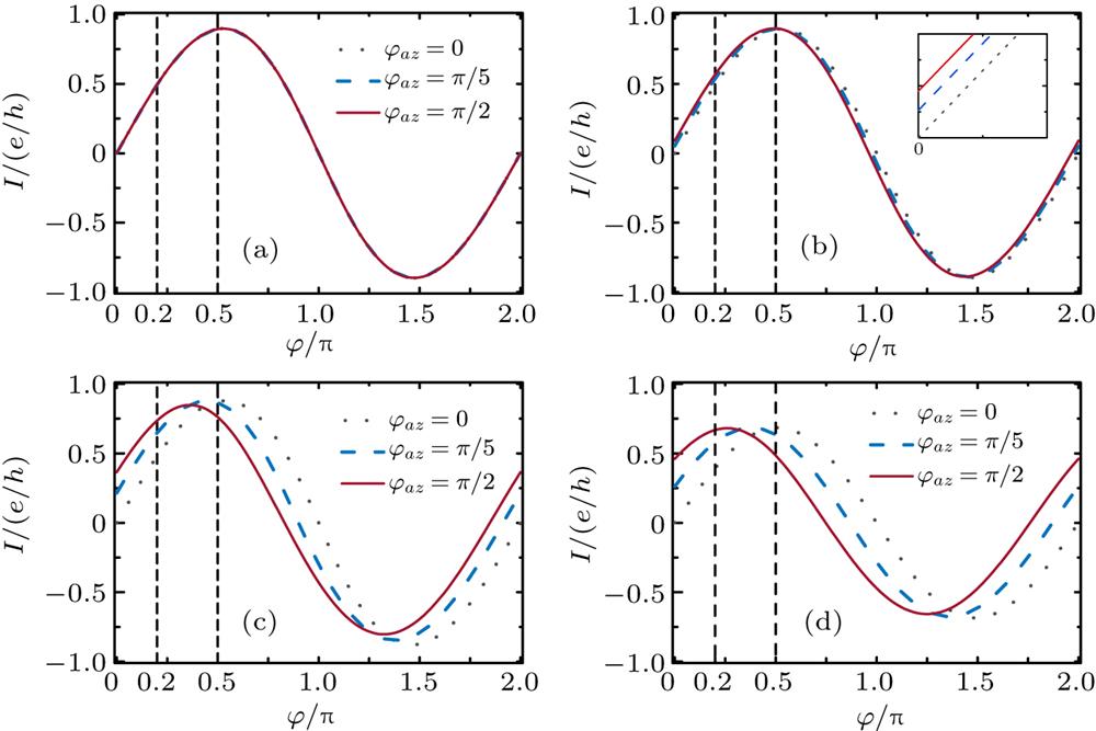
Fig. 2. Current–phase relations, i.e., the current I versus the superconducting phase difference φ with the magnetization M = 0 (a), 0.05 (b), 0.2 (c), and 0.35 (d). Different curves correspond to different azimuth angles φ_az = 0, π/5, and π/2. The vertical dashed lines mark φ = π/5 and π/2. The inset in (b) amplifies the current around φ = 0 to highlight the anomalous current. Other parameters are the nanoribbon width W = 80 and thickness of the domain wall L_dw = 3.

Fig. 3. Supercurrent I versus the azimuth angle φ_az, corresponding to φ = 0 (a), π/5 (b), π/2 (c), π (d), and 3π/2 (e). Curves in different colors represent different values of magnetization M = 0, 0.05, 0.2, and 0.35. All parameters unmentioned are the same as those in Fig. 2.

Fig. 4. Phase shift δ and amplitude A₁ versus the azimuth angle φ_az in QAHI-based Josephson junction, calculated from Eqs. (21) and (22). [(a), (b)] Curves with different magnetization M = 0, 0.05, 0.2, 0.35 and other parameters L_dw = 3 and W = 80. [(c), (d)] Curves with different widths W = 20, 40, 60, 80 and other parameters L_dw = 3 and M = 0.2.

Fig. 5. The maximum phase shift δ_max (a) and supercurrent amplitude A_m (b) versus magnetization M in the Bloch-type domain wall (φ_az = π/2). Different curves label different thicknesses of a domain wall L_dw = 10⁻⁵, 0.5, 1, 2, 3, and 4. All parameters unmentioned are the same as those in Fig. 2.

Fig. 6. The maximum phase shift δ_max (a) and amplitude of supercurrent A_m (b) versus magnetization M in the Bloch-type domain wall (φ_az = π/2). Different curves label different widths of junction W = 20, 40, 60, and 80. All parameters unmentioned are the same as those in Fig. 2.

Fig. 7. The maximum phase shift δ_max (a) and amplitude of supercurrent A_m (b) versus magnetization M in the Bloch-type domain wall (φ_az = π/2). Different curves label different paths with coefficients α = 0.6, 0.8, 1, 1.2, and 1.4. The inset in (b) shows the projection of magnetization in the y–z plane. All parameters unmentioned are the same as those in Fig. 2.

Fig. 8. (a) Schematic diagram for the QAHI-based Josephson junction with bare QAHI layers. The domain wall structure is gradually rotating along the x direction, plotted by vectors pointing the orientation of magnetization. Note: the illustration is not drawn to scale; in practice, the thickness of a domain wall L_dw is much smaller than the size of junction. The maximum phase shift δ_max (b) and amplitude of supercurrent A_m (c) versus magnetization M in the Bloch-type domain wall (φ_az = π/2). Different curves label the different numbers of the bare QAHI layer L_Q. All parameters unmentioned are the same as those in Fig. 2.

Fig. 9. Continuous transition from 0 junction to π junction in QAHI-based Josephson junction with bare QAHI layers. The supercurrent I versus the phase difference φ with (a) L_Q = 3 and (b) L_Q = 4 in the Bloch-type domain wall (φ_az = π/2). Different curves correspond to different magnetization M = 0,0.17,0.27,0.37 in (a) and M = 0,0.07,0.2,0.32 in (b). All parameters unmentioned are the same as those in Fig. 2.

Table 1. Symmetry operations on Hamiltonian. Here we take “–” to represent that the Hamiltonian term remains unchanged under the corresponding symmetry operation.