Light rays and waves on geodesic lenses

Lin Xu; Xiangyang Wang; Tomáš Tyc; Chong Sheng; Shining Zhu; Hui Liu; Huanyang Chen

doi:10.1364/PRJ.7.001266

Journals >Photonics Research >Volume 7 >Issue 11 >Page 1266 > Article

Photonics Research
Vol. 7, Issue 11, 1266 (2019)

Lin Xu^1、4、†, Xiangyang Wang^2、†, Tomáš Tyc^{3、5、†,*}, Chong Sheng², Shining Zhu², Hui Liu^2、6、*, and Huanyang Chen^1、7、*

Author Affiliations

¹Institute of Electromagnetics and Acoustics and Key Laboratory of Electromagnetic Wave Science and Detection Technology, Xiamen University, Xiamen 361005, China

²National Laboratory of Solid State Microstructures and School of Physics, Collaborative Innovation Center of Advanced Microstructures, Nanjing University, Nanjing 210093, China

³Department of Theoretical Physics and Astrophysics, Masaryk University, Kotlarska 2, 61137 Brno, Czech Republic

⁴Institutes of Physical Science and Information Technology & Key Laboratory of Opto-Electronic Information Acquisition and Manipulation of Ministry of Education, Anhui University, Hefei 230601, China

⁵e-mail: tomtyc@physics.muni.cz

⁶e-mail: liuhui@nju.edu.cn

⁷e-mail: kenyon@xmu.edu.cn

show less

DOI: 10.1364/PRJ.7.001266 Cite this Article Set citation alerts

Lin Xu, Xiangyang Wang, Tomáš Tyc, Chong Sheng, Shining Zhu, Hui Liu, Huanyang Chen. Light rays and waves on geodesic lenses[J]. Photonics Research, 2019, 7(11): 1266 Copy Citation Text

EndNote(RIS)

BibTex

Plain Text

show less

$AIs (upper row) and corresponding GLs (lower row) with rotational symmetry. In AIs, the center of each lens is marked with S. The position vector is denoted with r. The angle parameter θ is omitted for simplification because of rotational symmetry of AIs and GLs. Contour plots show refractive index profile of n(r). The presented AIs are Maxwell’s fish-eye lens (a), generalized Maxwell’s fish-eye lens with M=5 (b), extended invisible lens (c), and inverse invisible lens (d). The corresponding geodesic lenses are sphere (a), spindle with M=5 (b), Tannery’s pear (c), and truncated Tannery’s pear (d). On GLs, the axis of rotational symmetry is denoted by a dashed line, which connects north (N) pole and south (S) pole. ρ is the radial coordinate, and h(ρ) is the length measured along the meridian from N pole on the geodesic surface. Light rays starting from point A form closed trajectories shown in different colors. S poles are mapped from the centers S of AIs, while N poles correspond to the infinities of AIs. Dashed black circles of AIs are places with refractive index of unity at radius of r0, which are equivalent to those of GLs.$

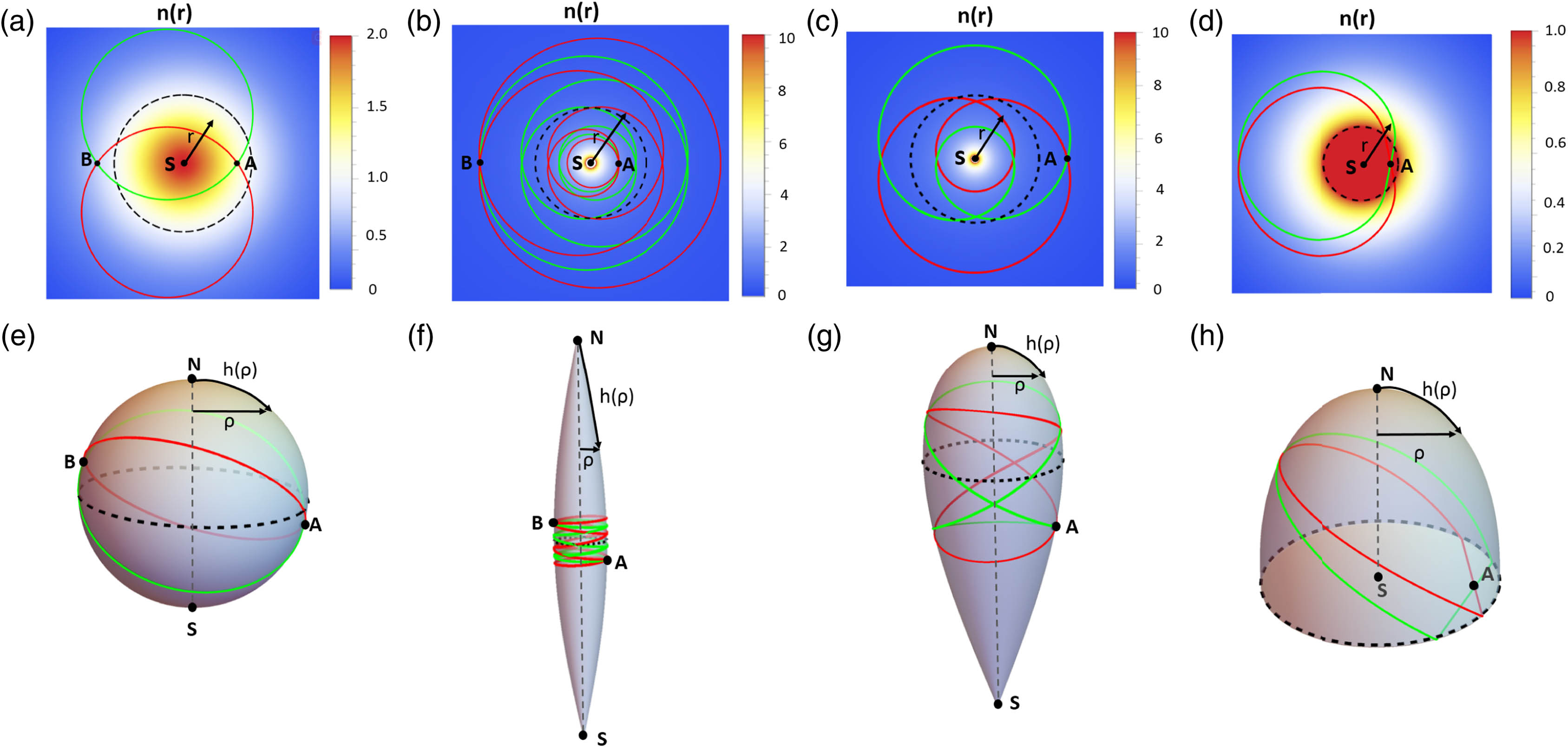
Fig. 1. AIs (upper row) and corresponding GLs (lower row) with rotational symmetry. In AIs, the center of each lens is marked with S. The position vector is denoted with r. The angle parameter θ is omitted for simplification because of rotational symmetry of AIs and GLs. Contour plots show refractive index profile of n(r). The presented AIs are Maxwell’s fish-eye lens (a), generalized Maxwell’s fish-eye lens with M=5 (b), extended invisible lens (c), and inverse invisible lens (d). The corresponding geodesic lenses are sphere (a), spindle with M=5 (b), Tannery’s pear (c), and truncated Tannery’s pear (d). On GLs, the axis of rotational symmetry is denoted by a dashed line, which connects north (N) pole and south (S) pole. ρ is the radial coordinate, and h(ρ) is the length measured along the meridian from N pole on the geodesic surface. Light rays starting from point A form closed trajectories shown in different colors. S poles are mapped from the centers S of AIs, while N poles correspond to the infinities of AIs. 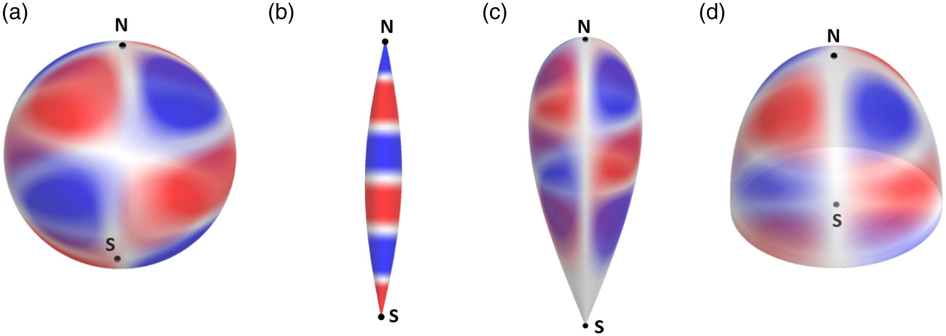Dashed black circles of AIs are places with refractive index of unity at radius of r0, which are equivalent to those of GLs.

Download full size | View in the Article

Fig. 2. Real part of the modes with different indices N and m: (a) ψ22 on sphere, (b) ψ50 on spindle, (c) ψ22 on Tannery’s pear, and (d) ψ22 on truncated Tannery’s pear.

Download full size | View in the Article

Fig. 3. Experimental setup and sample description. (a) Schematic of the observation and coupling scheme of the light to the geodesic lens. A laser beam is coupled to a 3D curved waveguide from the top and excites the rare-earth ions in the waveguide. The emitted fluorescent light at 615 nm is then collected by a CCD camera. (b) 3D curved waveguide morphology captured by a CCD camera when illuminated by white light. (c) Scanning electron microscope image of the 3D curved surface around the coupling grating (red dashed box) before spin coating. The cross structure corresponds to that displayed in (b) and is used to couple laser beams into the waveguide. (d) Scanning electron microscope image of the 3D curved surface with larger scale (blue dashed box) before spin coating. Based on this figure, one can get the accurate parameters of the 3D curved surface.

Download full size | View in the Article

Fig. 4. Optical measurements and fitting results of light rays in a spindle with M=5. (a) Fitting the shape of micro-structured metallic needle waveguide with a spindle. (b) Optical measurements on micro-structured metallic needle waveguide. (c) Enlarged drawing nearby the coupling source. (d) Fitting the light trajectory of micro-structured metallic needle waveguide with a spindle.

Download full size | View in the Article

Fig. 5. Sample fabrication process. (a) Position of straight silver wire, movement console (MC), and hydrogen flame. A straight silver wire is fixed on MC1 and MC2 and then put on a hydrogen flame at a proper position. (b) Metallic wire fusion process. The ends of the straight silver wire are pulled at speeds v1 and v2, and the silver wire gradually becomes tapered. (c) Two obtained metallic cones. The silver wire breaks into two metallic cones at some point.

Download full size | View in the Article

Fig. 6. (a) Sketch of a metallic waveguide. (b) Cross section of the metallic waveguide.

Download full size | View in the Article

Fig. 7. (a) Sketch of the coupling grating (yellow boxes). (b) SEM image of the metallic curved surface and the coupling grating (in red dashed box) before spin-coating process. (c) Grating coupling process and optical measurement of the sample. The yellow boxes in (a) show the coupling grating, the graded blue spot represents the exciting beam, and the blue arrows show the direction of the laser beam propagating in the waveguide. The coupling grating in (a) corresponds to the red dashed box in (b), which is fabricated before spin-coating process. The red dashed box region in (b) corresponds to the grating in (c), which is indicated by the red arrows.

Download full size | View in the Article

Fig. 8. Optical measurements and fitting results of light rays on a sphere. (a) CCD camera picture of micro-structured sphere waveguide. (b) Light trajectory on micro-structured sphere waveguide. (c) Fitting the light trajectory with a sphere.

Download full size | View in the Article

Lens	Refractive Index Profile	Geodesic Lens	Description of Geodesic Lens	Spectrum
Maxwell’s fish-eye lens	$n (r) = \frac{2}{1 + {(r / r_{0})}^{2}}$	Sphere	$h (ρ) = \arcsin (ρ)$	$\frac{ω_{N m} r_{0}}{c} = \sqrt{(N + m) (N + m + 1)} \approx N + m + 0.5$
Generalized Maxwell’s fish-eye lens	$n (r) = \frac{2 {(r / r_{0})}^{1 / M - 1}}{1 + {(r / r_{0})}^{2 / M}}$ , $M = 2, 3, 4, \dots$	Spindle	$h (ρ) = \arcsin (M ρ)$ , $M = 2, 3, 4, \dots$	$\frac{ω_{N m} r_{0}}{c} = \frac{\sqrt{(N + M \cdot m) (N + M \cdot m + 1)}}{M} \approx \frac{N + 0.5}{M} + m$
Extended invisible lens	$(r / r_{0}) n^{3 / 2} + (r / r_{0}) n^{1 / 2} - 2 = 0$	Tannery’s pear	$h_{1} (ρ) = - ρ + 2 \arcsin (ρ)$ , $h_{2} (ρ) = ρ + 2 \arcsin (ρ)$	$\frac{ω_{N m} r_{0}}{c} \approx \frac{N + 0.5}{2} + m$
Inverse invisible lens	$(r / r_{0}) n^{3 / 2} + (r / r_{0}) n^{1 / 2} - 2 = 0 for r > r_{0};$ $n = 1 for r < r_{0}$	Truncated Tannery’s pear	$h_{1} (ρ) = - ρ + 2 \arcsin (ρ)$ , $h_{2} (ρ) = 2 + π - ρ$	$\frac{ω_{N m} r_{0}}{c} \approx N + m + 0.5$

Table 1. Description of Four AIs and Corresponding GLs with Spectrum

Lin Xu, Xiangyang Wang, Tomáš Tyc, Chong Sheng, Shining Zhu, Hui Liu, Huanyang Chen. Light rays and waves on geodesic lenses[J]. Photonics Research, 2019, 7(11): 1266

Download Citation

EndNote(RIS)

BibTex

Plain Text

Set citation alerts for the article

Tools

Set citation alerts for the article

Save the article for my favorites

Paper Information