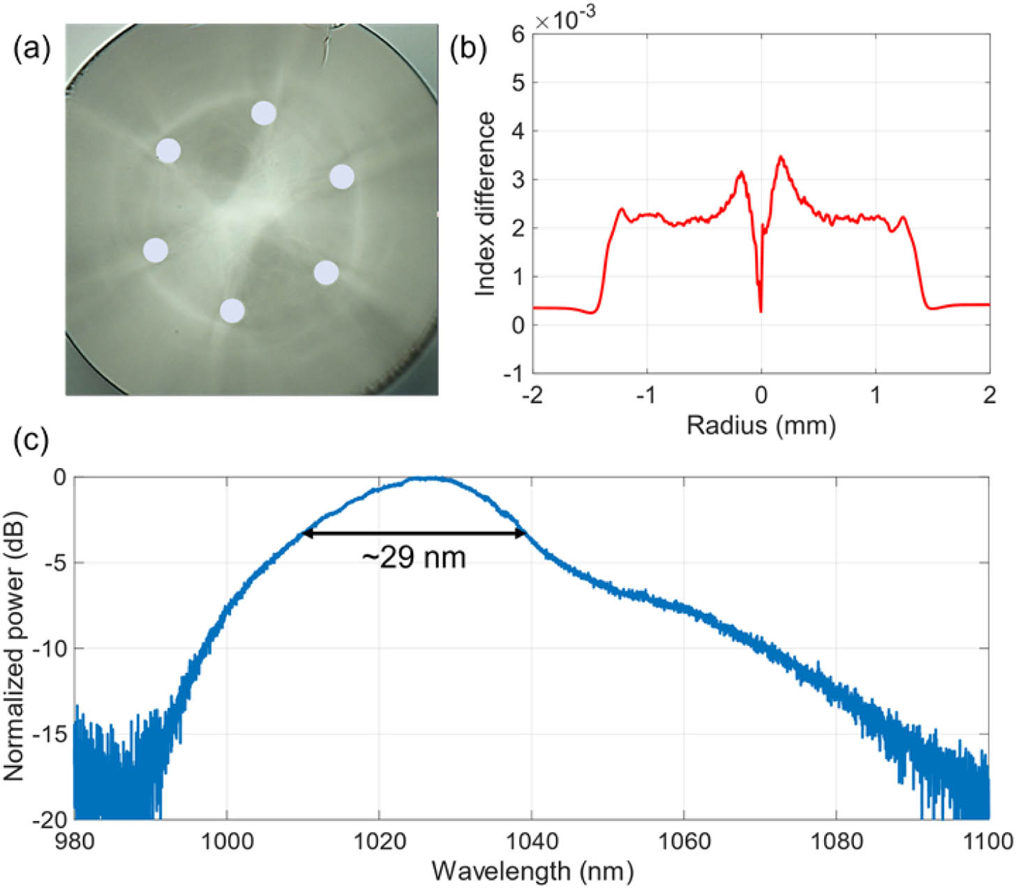
Fig. 1. Yb-doped six-core MCF. (a) Microscopic image of fiber cross-section. (b) Refractive index profile of the fabricated preform. (c) ASE spectrum of the MCF.

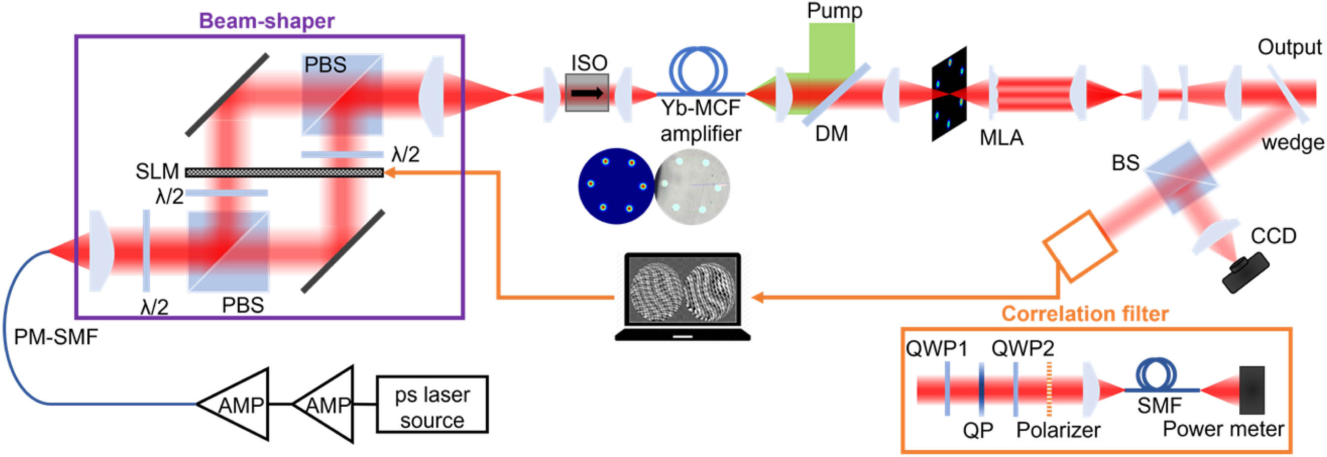
Fig. 2. Schematic of the experimental setup. AMP, amplifier; PM, polarization-maintaining; SMF, single-mode fiber; PBS, polarization beam splitter; λ/2, half-wave plate; ISO, isolator; DM, dichroic mirror; MLA, microlens array; BS, beam splitter; CCD, charge-coupled device; QWP, quarter-wave plate; QP, q-plate.

Fig. 3. Yb-MCF amplifier characterization. (a) Measured near-field intensity distribution of the MCF output. (b) Average output power versus the launched pump power. (c) Measured spectra of the seed and of the amplified output at an average output power of ∼12.3  W [resolution is  0.5  nm (upper) and 0.02  nm (lower)]. (d) Temporal pulse shapes of the seed and the amplified output at ∼12.3  W.

Fig. 4. Generation of linearly polarized Gaussian beams. (a) Far-field beam profiles without beam shaping. (b) Simulated far-field intensity distribution when all cores are in-phase. (c), (d) Experimentally measured far-field Gaussian beam profiles at the peak power of ∼8.14  kW with the orthogonal polarization states.

Fig. 5. Generation of CV beams. (a) Simulated far-field intensity distribution when the polarization orientations of the six beamlets are set as per the arrow directions in (b). (c) Experimentally measured radially polarized output beam profile with a peak power of ∼11.4  kW, and the two-lobe patterns when the beam is passed through a linear polarizer at different orientations (white arrows). (d) Experimentally measured azimuthally polarized beam profile (at ∼10  kW) and the two-lobe patterns after passing through the linear polarizer.

Fig. 6. Generated OAM beams (first order). (a), (d) Experimentally measured output beam profiles with a peak power of ∼10.7  kW and the topological charge of ±1, respectively, as well as the corresponding intensity distributions after the beam was passed through a rotatable linear polarizer. (b), (e) Measured spiral interference fringes for the generated OAM beams shown in (a) and (d). (c), (f) 1D intensity profiles across the beam center fitted with an incoherent superposition of the LP01 mode and the OAM mode.

Fig. 7. Generation of OAM beams (second order). (a) Simulated far-field distribution when the relative phase of the six beamlets is set to the value given in (b). (c), (d) Experimentally measured beam profiles with a peak power of ∼14.4  kW and the topological charge of ±2, respectively, as well as the corresponding intensity distributions after passing through a rotatable linear polarizer. (e), (f) Measured spiral interference fringes for the generated OAM beams shown in (c) and (d).

Fig. 8. Numerical analysis on the factors affecting the combining efficiency and far-field beam shape. (a) Calculated combining efficiency of the first-order OAM as a function of MLA defocus with different mode composition (weight w of LP01 mode) of the MCF output. (b) Combining efficiency of the combined Gaussian and OAM beams with different MLA shifts in the CBC setup. (c) Combining efficiency of the combined beams with different power distributions of the MCF beamlets. (d) Near-field and far-field intensity profiles under different power distributions [A–D shown in (c)].