


 (K)
(K) (K)
(K) (%) – eight slabs
 ) – eight slabs
 ) – eight slabs
Antonio Lucianetti, Magdalena Sawicka, Ondrej Slezak, Martin Divoky, Jan Pilar, Venkatesan Jambunathan, Stefano Bonora, Roman Antipenkov, and Tomas Mocek. Design of a kJ-class HiLASE laser as a driver for inertial fusion energy[J]. High Power Laser Science and Engineering, 2014, 2(2): 02000e13
- High Power Laser Science and Engineering
- Vol. 2, Issue 2, 02000e13 (2014)
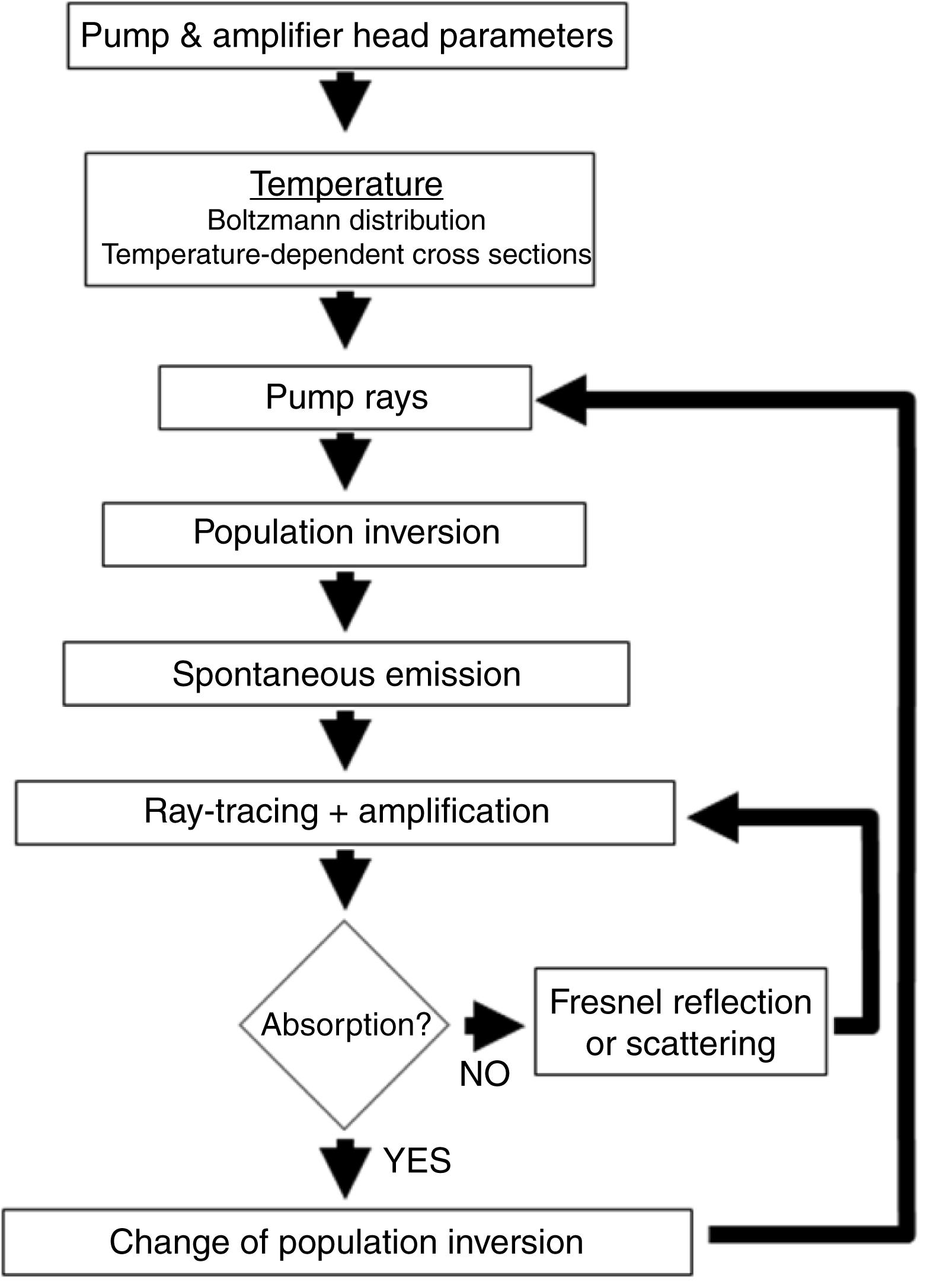
Fig. 1. A schematic flow diagram of the model.
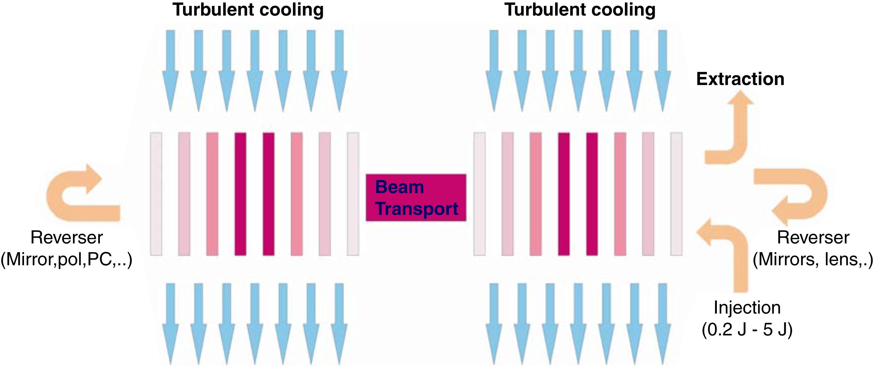
Fig. 2. Block diagram of the HiLASE kJ laser (two-head configuration).
Fig. 3. Block diagram of the HiLASE kJ laser (single-head configuration).
Fig. 4. The time-resolved extractable energy in the HiLASE slab for different pump intensities ( K).
K).
K). Fig. 5. The time-resolved extractable energy in the HiLASE slab for different pump intensities ( K).
K).
K). Fig. 6. The time-resolved extractable energy in the HiLASE slab for different pump intensities ( K).
K).
K). Fig. 7. The extractable energy as a function of the operating temperature for different pump intensities.
Fig. 8. The storage efficiency as a function of the operating temperature for different pump intensities.
Fig. 9. The evolution of the extracted energy for different input energies at 200 K (two heads, 20% optical losses per round trip pass). The total pump intensity was  .
.
. Fig. 10. The evolution of the extracted energy for different input energies at 200 K (two heads, 16% optical losses per round trip pass). The total pump intensity was  .
.
. Fig. 11. The evolution of the extracted energy for different input energies at 200 K (one head, 18% optical losses per round trip pass). The total pump intensity was  .
.
. Fig. 12. The evolution of the extracted energy for different input energies at 200 K (one head, 10% optical losses per round trip pass). The total pump intensity was  .
.
. Fig. 13. The MIRO model used to calculate the temporal shape, spatial shape, and B integral of the HiLASE kJ laser.
Fig. 14. Input, output, and desired temporal profiles of the MIRO model for the HiLASE kJ laser.
Fig. 15. The evolution of the B integral and accumulated B integral upon beam propagation in the HiLASE kJ laser.
Fig. 16. (a) Beam profile, (b) and (c) phase after subtraction of defocus and tilt of the output beam.
Fig. 17. (a) The stress- and temperature-induced OPD after a single pass through the laser head (after one pass through eight slabs). (b) The depolarization of the beam after a single pass through the head caused by stress-induced birefringence. The  :YAG cladding thickness was 20 mm.
:YAG cladding thickness was 20 mm. Fig. 18. The geometry and zone layout used for heat deposition modeling in the HiLASE amplifier slab.
Fig. 19. (a) The calculated OPD and (b) the depolarization loss due to eight slabs. A 3 mm layer of undoped YAG and two 25 mm Cr:YAG layers of cladding with different doping levels were added around the gain medium.
Fig. 20. The actuator layout of the DM.
Fig. 21. Residual rms values of the OPD as a function of the stroke after correction by the DM.
Fig. 22. (a) The output wavefront calculated in MIRO and shown in Figure 16 (a) after subtraction of tilt and defocus. (b) The residual wavefront after correction by the DM with  actuators (
 ,
,  ).
).
actuators (, ). Fig. 23. (a) Far field with ideal flat wavefront. (b) Far-field image before correction by the DM. (c) Far-field image after correction with  actuators (
 ,
,  ).
).
actuators (, ). Fig. 24. The SHG efficiency for different LBO thickness values.
Fig. 25. The THG efficiency for different LBO thickness values.
|
Table 1. The Gain Medium and Cladding Dimensions used for Simulation of HiLASE Square Amplifiers.
|
Table 2. Thermal Results for HiLASE Square Amplifiers (Single, Enlarged Single, and Double Clad).

Set citation alerts for the article
Please enter your email address
© Copyright 2018-2021 | Chinese Laser Press. All Rights Reserved 沪ICP备15018463号-20