
Licheng Sun, Tinghao Liu, Xing Fu, Yading Guo, Xiaojun Wang, Chongfeng Shao, Yamin Zheng, Chuang Sun, Shibing Lin, Lei Huang. 1.57 times diffraction-limit high-energy laser based on a Nd:YAG slab amplifier and an adaptive optics system[J]. Chinese Optics Letters, 2019, 17(5): 051403
- Chinese Optics Letters
- Vol. 17, Issue 5, 051403 (2019)
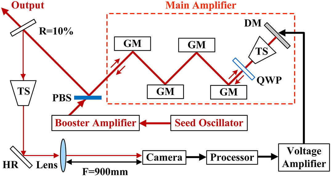
Fig. 1. Schematic of the Nd:YAG slab amplifier with an AO configuration. HR, high reflection mirror; PBS, polarization beam splitter; GM, gain module; QWP, quarter-wave plate; TS, telescope.
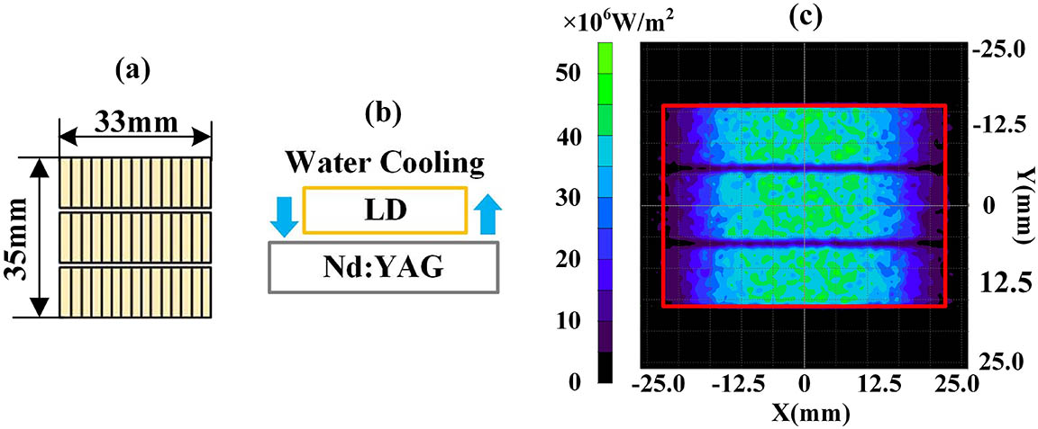
Fig. 2. (a) LD array. (b) Gain module without shaping optics. (c) Simulation pump intensity distribution in a Nd:YAG slab without shaping optics. The red rectangle represents the laser beam in a Nd:YAG slab.
Fig. 3. Experimental results with the
Fig. 4. Actuators distribution of the DM and the
Fig. 5. Correction result of the defocus distributed in a
Fig. 6. Correction result of the defocus distributed in a
Fig. 7. HBQ after correction with different beam arrays.
Fig. 8. (a) Gain module with a pump-light homogenizer. (b) Simulation pump intensity distribution in a Nd:YAG slab with a pump-light homogenizer.
Fig. 9. Experimental results with the pump-beam array. Near-field intensity distribution (a) before correction,
|
Table 1. PV Value, RMS Value, and HBQ of the Defocus Distributed in Different Arrays After Correction

Set citation alerts for the article
Please enter your email address
© Copyright 2018-2021 | Chinese Laser Press. All Rights Reserved 沪ICP备15018463号-20