Distributed Brillouin frequency shift extraction via a convolutional neural network

Yiqing Chang; Hao Wu; Can Zhao; Li Shen; Songnian Fu; Ming Tang

doi:10.1364/PRJ.389970

Abstract

Distributed optical fiber Brillouin sensors detect the temperature and strain along a fiber according to the local Brillouin frequency shift (BFS), which is usually calculated by the measured Brillouin spectrum using Lorentzian curve fitting. In addition, cross-correlation, principal component analysis, and machine learning methods have been proposed for the more efficient extraction of BFS. However, existing methods only process the Brillouin spectrum individually, ignoring the correlation in the time domain, indicating that there is still room for improvement. Here, we propose and experimentally demonstrate a BFS extraction convolutional neural network (BFSCNN) to retrieve the distributed BFS directly from the measured two-dimensional data. Simulated ideal Brillouin spectra with various parameters are used to train the BFSCNN. Both the simulation and experimental results show that the extraction accuracy of the BFSCNN is better than that of the traditional curve fitting algorithm with a much shorter processing time. The BFSCNN has good universality and robustness and can effectively improve the performances of existing Brillouin sensors.

1. INTRODUCTION

Distributed optical fiber sensors can realize a variety of physical quantity measurements at each point along an optical fiber [1]. Among them, distributed optical fiber Brillouin sensors are able to obtain the temperature and strain along a fiber by measuring the distributed Brillouin frequency shift (BFS) [2]. This technology is widely used in the monitoring of large structures, such as bridges and dams, and long-distance temperature measurements for pipelines and tunnels [3]. The distributed BFS is generally obtained by measuring the Brillouin gain spectrum (BGS) of an optical fiber. Since the BGS theoretically satisfies a Lorentzian shape, the BFS can be obtained by performing Lorentzian curve fitting (LCF) on the BGS, which is measured at a limited frequency sampling interval [4]. However, the accuracy of LCF is easily affected by the initial values of the fitting parameters [5,6]. When the signal-to-noise ratio (SNR) is low, improper initial values may lead to a serious error in the fitting result. In addition, the curve fitting algorithm is iterative. Therefore, its processing time is relatively long, which affects the response time of the sensor. To improve the sensing performance, a more accurate and efficient BFS extraction method is needed.

Recently, other methods, such as cross-correlation [5,7], principal component analysis [8], and machine learning methods, have been proposed to analyze the BGS [9–13]. Although these algorithms can achieve better results than LCF under certain conditions, they also have some drawbacks. The cross-correlation method calculates the frequency difference to obtain the BFS by convolving the ideal BGS with the measured BGS. It has a higher requirement for the frequency sampling interval than LCF. Clustering and classification algorithms such as principal component analysis and support vector machine have shown good performance for BFS extraction [8–11]. Nevertheless, these algorithms have a trade-off problem between the number of principal components or classes and capability. The accurate extraction of BFS depends on classes or subdivided principal components and large storage databases. Alternatively, artificial neural networks have also been proven effective [12,13]. However, neural networks are usually trained based on specific data. Retraining or fine-tuning is required to accommodate different actual data, which significantly affects its application potential. In addition, all of the above methods are designed to analyze only a single BGS at a time to estimate its corresponding BFS. However, the measured result of a distributed Brillouin sensor is natural two-dimensional (2D) data with both time-domain and frequency-domain information. Existing methods only consider the frequency-domain characteristics of the data and do not take advantage of its time-domain correlation, indicating that there is still room for improvement [14].

To achieve more efficient BFS extraction with better universality and robustness, a distributed BFS extraction convolutional neural network (BFSCNN) is proposed in this paper. Multilayer 2D convolution is used to analyze the frequency and time features of the measured data and realizes an end-to-end transformation from the 2D data to a one-dimensional (1D) distributed BFS. To adapt the BFSCNN to different instruments and application scenarios, a large number of ideal BGSs with random BFSs, spectral widths (SWs), and SNRs are generated by simulation. These BGSs are randomly combined into 2D data as the input of the BFSCNN, and the corresponding distributed BFS is used as the training target. By optimizing the network structure, training data, and training process, the BFSCNN realizes a high-precision distributed BFS extraction for both the simulation and experiment data. In addition, the proposed BFSCNN is a full convolutional network that can fully utilize the parallel computing power of the hardware and effectively reduce the processing time.

Sign up for Photonics Research TOC. Get the latest issue of Photonics Research delivered right to you！Sign up now

2. MATERIALS AND METHODS

A. LCF

The most general method to obtain the BFS is the LCF because the BGS theoretically satisfies a Lorentzian shape: $g (v) = \frac{g_{B}}{1 + {(\frac{v - v_{B}}{Δ v_{B} / 2})}^{2}},$ (1)where $g_{B}$ is the Brillouin gain coefficient, $Δ v_{B}$ is the full width at half-maximum of the spectrum, which is the SW, and $v_{B}$ represents the BFS. Before fitting, the initial values of these parameters should be set. The maximum value of the BGS is assigned to $g_{B}$ , and its corresponding frequency is assigned to $v_{B}$ . The initial value of the SW is estimated by calculating the frequency range, where the intensity exceeds half of the maximum gain.

Starting with the initial values, the least squares method is used to find parameters to best fit Eq. (1) iteratively. That is, for a set of measured data ( $v_{i}, g_{i}$ ), the purpose of the method is to find the parameters $\hat{a}$ so that the sum of the square error is minimized: $\hat{a} \equiv {argmin}_{a} \sum_{i = 1}^{m} {[g_{i} - g (v_{i}; a)]}^{2} .$ (2)The Levenberg–Marquardt algorithm (LMA) is employed to solve this nonlinear least squares problem [6,15]. The LMA combines the advantages of the Gauss–Newton algorithm and gradient descent method to obtain better robustness. Based on the LMA, the parameters are continuously evolved through iteration until the iteration step is less than the stopping criteria, which is set to $10^{- 8}$ .

B. Proposed BFSCNN

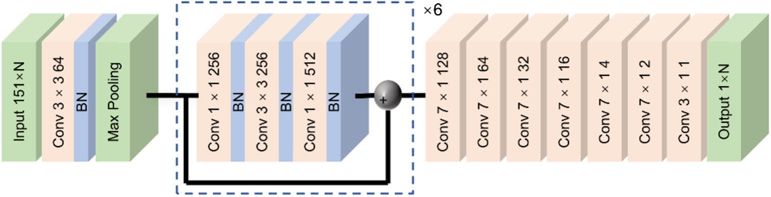
As illustrated in Fig. 1, the proposed BFSCNN consists of three parts. The first part starts with an input layer of $151 \times N \times 1$ . The number 151 represents the number of frequency sampling points, which is a general choice considering the sampling time. $N$ means the number of input BGS traces. It is important to note that there is a one-to-one correspondence between the input BGS and the output BFS. Therefore, the length of the signal at the time dimension should not be reduced over the BFSCNN during the process. The input data are first processed by 64 convolutional filters (Conv) of size $3 \times 3$ to generate 64 feature maps. Convolution operation can extract different features from images using different convolutional filters [16]. In shallow layers, the elementary features such as edges, end points, and corners are obtained. These features are then combined in higher layers to learn characteristics of the input. However, it is hard to train a network with only Conv, so batch normalization (BN) is introduced to help the training process. By normalizing the layer’s input without changing what the previous layer represents, BN can reduce the internal covariate shift problem in the training process [17]. And the rectified linear unit (ReLU) activation function is adopted to add nonlinear factors [18]. After that, a max pooling layer with a spatial extent of $2 \times 1$ and a step size of $2 \times 1$ is used to reduce the size of the feature map. This down-sampling process replaces each spatial extent with its maximum value, which helps the BFSCNN to focus on more valuable information.

Architecture of the proposed BFSCNN.

Figure 1.Architecture of the proposed BFSCNN.

The second part is an 18-layer residual subnetwork [19]. There are six ResBlocks with the structure of $Conv (1 \times 1) - Conv (3 \times 3) - Conv (1 \times 1)$ . The $3 \times 3$ convolution kernels are used to perceive features in both the time and frequency domains. The $1 \times 1$ convolution kernels are employed to introduce more nonlinearly with the ReLU. All convolutional layers in the first two parts are in the same padding mode to ensure that the number of points in the time dimension is $N$ .

The third part is a plain net that aims to obtain the 1D BFS from the 2D data. Therefore, $M \times 1$ convolution kernels without padding are used. After testing and optimization, a seven-layer scheme that utilizes $7 \times 1$ and $3 \times 1$ convolution kernels is chosen, through which the number of points in the frequency dimension gradually decreases. Finally, the output size is $1 \times N$ , corresponding to the BFSs for N input BGSs. The number of input BGS traces is not fixed because the BFSCNN can traverse the input two-dimensional data and output corresponding BFSs.

C. Data Preparation

To ensure the efficient operation of the BFSCNN, the input data must be normalized as shown in Fig. 2. First, the maximum value of the BGS is transformed to 1. The BFS is normalized according to the frequency sweep range: ${BFS}_{N} = \frac{BFS - f_{\min}}{f_{\max} - f_{\min}},$ (3)where $f_{\max}$ and $f_{\min}$ represent the maximum and minimum values of the frequency sweep range, respectively. The SW is also normalized according to the frequency sweep range:

Figure 2.Normalized simulation BGSs. BGS1: $BFS = 20 %$ , $SW = 13 %$ , $SNR = 20 dB$ ; BGS2: $BFS = 50 %$ , $SW = 30 %$ , $SNR = 15 dB$ ; BGS3: $BFS = 73 %$ , $SW = 50 %$ , $SNR = 10 dB$ .

{SW}_{N} = \frac{SW}{f_{\max} - f_{\min}} .

(4)

D. Training Process

Simulated BGSs are used to train the BFSCNN. The BGSs are generated as Lorentzian curves with a random BFS and SW. To further enhance the robustness, Gaussian white noise is added to the ideal BGSs with a random SNR. The SNR is defined as the ratio between the maximum gain of a signal and the power of noise. According to the general Brillouin sensing data, the random range of the BFS is set to 5% to 95%, the range of the SW is 10% to 50%, and the range of the SNR is 5 to 20 dB. The random values of BFS, SW, and SNR are uniformly distributed. By combining the simulated BGSs randomly, 2D data are generated as the input of the BFSCNN, and its corresponding distributed BFS is used as the training target as shown in Fig. 3.

Figure 3.Simulation data used for training. (a) Simulation BGSs of random parameters; (b) corresponding BFSs.

The parameters of the BFSCNN are initialized randomly as a uniform distribution. Then, the optimization function Adam is employed to optimize the parameters according to the training data [20]. For each iteration, the training data go through forward propagation as shown in Eq. (5). Then, the backward propagation of the loss value is calculated according to Eq. (6). Finally, the network parameters are updated based on Eq. (7): $x^{l} = {\begin{cases} 1, & l = 1 \\ , \\ σ (w^{l} x^{l - 1} + b^{l}), & l = 2 to L \end{cases},$ (5) $δ^{l} = {\begin{cases} MSE (z^{l}), & l = L \\ , \\ δ^{l + 1} * rot 180 (w^{l + 1}) \circ σ^{'} (z^{l}), & l = L - 1 to 2 \end{cases},$ (6) $θ_{t + 1}^{l} = θ_{t}^{l} - α \frac{{\hat{m}}_{t}}{\sqrt{{\hat{v}}_{t} + ε}},$ (7)where $x^{l}$ represents the output of the $l$ th layer in the forward propagation and $δ^{l}$ represents the gradient of the $l$ th layer in backward propagation. $θ^{l}$ refers to the parameters of the $l$ th layer, including weight $w$ and bias $b$ . $σ$ and MSE are the activation function and loss function, respectively. The symbol $\circ$ in Eq. (6) represents the Hadamard product. In Eq. (7), ${\hat{m}}_{t}$ and ${\hat{v}}_{t}$ are bias-corrected first moment and second raw estimations in Adam, respectively. In addition, $a$ is the learning rate.

The BFSCNN is trained for 22 epochs with a mini-batch size of 8. For each epoch, the parameters of BFSCNN is updated 375 times using 672,000 BGSs. For each update, $224 \times 8$ BGS traces are used, which is constrained by the memory size of GPU. The learning rate starts from 0.001 and gradually decreases with a decay of 0.0001 over each update. It takes approximately 2 h and 53 min to complete the training process based on a Python environment running on a computer with an AMD Ryzen 1950X 16-core processor and an Nvidia GeForce GTX 1080 GPU.

E. Experimental Setup

To demonstrate the validation of the trained BFSCNN on the actual distributed Brillouin sensors, a Brillouin optical time-domain analyzer (BOTDA) is set up to measure the distributed BGS data of a stand single-mode fiber that is approximately 25 km long. As shown in Fig. 4, the output of a narrow linewidth laser at 1550 nm is split into two branches through a 3 dB coupler. The probe light in the upper branch is modulated by an electro-optic modulator (EOM) operated in carrier-suppression mode to produce sidebands. The EOM is driven by an MS to control the frequency of the sidebands. Then, the probe passes through a polarization switch (PS) and launches into one end of the fiber. The output polarization state of the PS is controlled by an arbitrary function generator (AFG) to mitigate the polarization effects.

Figure 4.Experimental setup of the BOTDA system. EOM, electro-optic modulator; MS, microwave synthesizer; PS, polarization switch; FUT, fiber under test; SOA, semiconductor optical amplifier; AFG, arbitrary function generator; EDFA, erbium-doped fiber amplifier; BPF, bandpass filter; BVTF, bandwidth-variable tunable filter; PD, pin photodetector.

In the lower branch, an SOA driven by the AFG is exploited to generate optical pump pulses with a high extinction ratio ( $> 50 dB$ ). After amplification by an erbium-doped fiber amplifier (EDFA), the pump pulses are launched into the other end of the fiber through a circulator. Due to the stimulated Brillouin scattering effect, a part of the energy of the high-frequency pump light is transferred to the low-frequency probe light. Finally, the Brillouin-amplified probe wave is obtained through a BVTF and eventually detected by a 125 MHz PD. By continuously sweeping the frequency difference between the pump and probe light around the local BFS, the distributed BGS is obtained. The frequency scanning range is from 10.6 to 10.9 GHz at a step of 2 MHz, and the time-domain sampling rate is 250 MSa/s.

3. RESULTS AND DISCUSSION

To fully demonstrate the performance of the proposed BFSCNN, first, simulated ideal BGSs with different parameters are generated to verify the universality and robustness of the BFSCNN to various SNRs, BFSs, and SWs. Then, the actual measured distributed BGS is used for testing. These data are processed using the LCF and the trained BFSCNN to compare their performances.

A. Simulation Results

The root-mean-square error (RMSE) and standard deviation (SD) are used as evaluation parameters to compare the performances of the LCF and BFSCNN. As shown in Eq. (8), the RMSE characterizes the difference between the extracted BFS and its true value. The SD characterizes the dispersion of the extracted BFS as Eq. (9): $RMSE = \sqrt{\frac{1}{N} \sum_{i = 1}^{N} {(y - \hat{y})}^{2}},$ (8) $SD = \sqrt{\frac{1}{N} \sum_{i = 1}^{N} {(y - \bar{y})}^{2}},$ (9)where $y$ and $\hat{y}$ are the predicted and true BFSs, respectively, and $\bar{y}$ is the average of the predicted BFSs.

First, the performance of the BFSCNN at different SNRs is analyzed. The SW of the simulated BGSs is fixed at 25%, and the BFS is fixed at 30%. For each SNR in Table 1, 4480 noisy BGSs are generated by adding Gaussian white noise. As shown in Figs. 5(a) and 5(b), the RMSE and SD decrease as the SNR increases. The RMSE of the BFS extracted by the BFSCNN is better than that extracted by the LCF when the SNR is lower than 16 dB. A similar trend is found in the SD when the SNR is lower than 19 dB. By utilizing the 2D information of the BGSs, the BFSCNN can extract the BFS from the noisy data more accurately. Since the simulated BGSs are generated based on the Lorentzian shape, the LCF can achieve better results when the SNR is high.

Parameters	Range	Interval
SNR	5–19 dB	2 dB
BFS	10%–90%	5%
SW	10%–50%	5%

Table 1. Test Parameters

View all Tables

Figure 5.Normalized BFS RMSE and SD of the simulation data. (a) Normalized RMSE and (b) SD for different SNR data; (c) normalized RMSE and (d) SD for different BFS data; (e) normalized RMSE and (f) SD for different SW data.

To show the effects of the BFSCNN on different BFS data, the SW and SNR are chosen to be 25% and 11 dB, respectively. For each BFS in Table 1, 4480 BGSs are simulated for testing. As shown in Figs. 5(c) and 5(d), the processing results of the BFSCNN are better than those of the LCF for all cases. In addition, the BFSCNN has good consistency for different BFS data. However, when the BFS approaches the edge of the scanning range, the results using the LCF significantly deteriorate. This means that the BFSCNN has a higher tolerance for the incompleteness of the BGS and can achieve high-precision BFS extraction with less information.

BGSs with various SWs are also simulated, while the SNR and BFS are fixed at 11 dB and 25%, respectively. As shown in Figs. 5(e) and 5(f), it is harder to extract the BFS accurately via both methods when the SW increases. The results of the BFSCNN are always better than those of the LCF. For the LCF results, the changes in RMSE and SD with SW are basically consistent. However, the results obtained by the BFSCNN have less deterioration in the SD when the SW is large. Because the BFSCNN exploits the time-domain characteristics of the data, there is a correlation between adjacent BGSs, which causes the SD to be small.

To compare the performances of the BFSCNN and LCF more comprehensively, 4480 BGSs are simulated for each case in Table 1. We subtract the BFS RMSE using the BFSCNN from that of the result using the LCF and plot the differences in Fig. 6(a). Analogously, Fig. 6(b) shows the SD differences. Positive results are shown in blue, indicating that the RMSE or SD using the LCF is larger than that using the BFSCNN. Red indicates that the BFSCNN performs worse than the LCF in that case. In addition, the images with darker tones represent larger performance differences. The results indicate once again that the BFSCNN can extract the BFS more accurately when the SNR is low, and the correlation between different BGSs is stronger under this algorithm than the LCF. In the cases of low SNR, the values near the edges in the subgraphs are smaller, which indicates that the BFSCNN is more robust to the BGS than the LCF and can handle more extreme cases.

Figure 6.Performance differences in BFSs extracted by the LCF and BFSCNN. (a) Normalized BFS RMSE using the LCF minus the normalized BFS RMSE using the BFSCNN for different simulation data. (b) Normalized BFS SD using the LCF minus the normalized BFS SD using the BFSCNN for different simulation data.

B. Experimental Results

Figure 7(a) shows the measured distributed BGSs when the pump pulse width is 40 ns and the average time is 32. It contains 62,000 BGS traces. They are processed by the BFSCNN and LCF, and the extracted BFSs are shown in Fig. 7(b). The values of the extracted BFSs are almost the same with some fluctuation. As the SNR decreases with distance, the fluctuation range becomes more severe. The fluctuation is weaker when using the BFSCNN than when using the LCF. However, the magnitude of the fluctuation is generally not used directly to judge the accuracy of BFS. Because the true BFS of the fiber is unknown, the fluctuation may be caused by temperature and strain.

Figure 7.Measurement results when the pump pulse width is 40 ns and the average time is 32. (a) Measured BGSs along an optical fiber; (b) distributed BFSs extracted by LCF and BFSCNN.

Here we use uncertainty as the basis for evaluating the performance of the extraction algorithms [4]. The distributed BGSs of the same fiber are continuously measured, and the data are processed by the BFSCNN and LCF. The uncertainty is defined as the quadratic fitted trace of the SD of the continuous extracted BFSs. To illustrate the universality and robustness of the proposed BFSCNN, several experiments are performed with different average times and pulse widths. Average times of 4 and 32 and pulse widths of 20, 30, and 40 ns are selected to achieve a large SNR range and SW variation. As shown in Fig. 8, the BFSCNN performs better than the LCF in almost all cases. When the uncertainty reaches below 0.4 MHz, the BFSCNN still has certain advantages, which verifies the conjecture in the simulation section: the BFSCNN may work better than the LCF for actual BGS even when the SNR is high.

Figure 8.BFS uncertainty as a function of fiber length. BFS uncertainty traces when the pump pulse width is (a) 20 ns, (b) 30 ns, and (c) 40 ns.

The spatial resolution is a key parameter for distributed Brillouin sensors and is defined as the fiber length of the BFS transition region between 10% and 90% of the peak frequency. To investigate whether the spatial resolution is affected by the BFSCNN, approximately 100 m of the fiber end is placed in a temperature-controlled chamber and heated to 50°C, while the rest of the fiber is at room temperature. Figure 9 shows the BFSs extracted by the LCF and BFSCNN when the pump pulse width is 40 ns and the average time is 32. The BFSs obtained by the two methods are basically the same in the transition region. Because the BFS of the training data varies randomly, the BFSCNN can adapt to arbitrary data without changing the spatial resolution.

Figure 9.Extracted BFSs along the optical fiber when the fiber end is heated. The inset image shows the BFS profiles around the start of the heat section.

C. Processing Time

For distributed Brillouin sensors, data-processing time is one of the key factors affecting the system response time. Especially for high-speed acquisition systems, the extraction time of LCF has become a bottleneck [21,22]. It takes approximately 0.129 s for the BFSCNN to process 1000 BGSs based on the Python environment running on the same computer for training. For the same data and operating environment, the LCF takes approximately 0.814 s, which is much longer than that of the CNN. It should be pointed out that the results of previous articles are generally running on MATLAB software. Therefore, the LCF processing time using MATLAB is also given as a reference here, which is approximately 12.14 s.

4. CONCLUSIONS

In this paper, a BFSCNN is proposed for the BFS extraction of distributed Brillouin sensors. Because of the full convolutional structure, the BFSCNN can obtain the distributed BFS directly from the measured 2D distributed BGSs. By making full use of the information of the 2D data, the BFSCNN achieves better BFS extraction accuracy than the traditional LCF. Both the simulation and experimental results confirm that the BFSCNN has better universality and robustness. Due to the comprehensive analysis of adjacent BGSs, the uncertainty of the BFS obtained by the BFSCNN has been significantly improved. In addition, the processing time of the BFSCNN is much shorter thanks to its suitable net structure for parallel computation.

The proposed BFSCNN can be applied to any distributed Brillouin sensor and effectively improve the performance with no hardware modification. We believe that the extraction accuracy and processing time could be further improved with optimized network structure and training dataset.

References

[1] P. Lu, N. Lalam, M. Badar, B. Liu, B. T. Chorpening, M. P. Buric, P. R. Ohodnicki. Distributed optical fiber sensing: review and perspective. Appl. Phys. Rev., 6, 041302(2019).

[2] A. Denisov, M. A. Soto, L. Thévenaz. Going beyond 1000000 resolved points in a Brillouin distributed fiber sensor: theoretical analysis and experimental demonstration. Light Sci. Appl., 5, e16074(2016).

[3] X. Bao, L. Chen. Recent progress in Brillouin scattering based fiber sensors. Sensors, 11, 4152-4187(2011).

[4] M. A. Soto, L. Thévenaz. Modeling and evaluating the performance of Brillouin distributed optical fiber sensors. Opt. Express, 21, 31347-31366(2013).

[5] M. A. Farahani, E. Castillo-Guerra, B. G. Colpitts. Accurate estimation of Brillouin frequency shift in Brillouin optical time domain analysis sensors using cross correlation. Opt. Lett., 36, 4275-4277(2011).

[6] C. Zhang, Y. Yang, A. Li. Application of Levenberg-Marquardt algorithm in the Brillouin spectrum fitting. 7th International Symposium on Instrumentation and Control Technology: Optoelectronic Technology and Instruments, Control Theory and Automation, and Space Exploration, 71291Y(2008).

[7] M. A. Farahani, E. Castillo-Guerra, B. G. Colpitts. A detailed evaluation of the correlation-based method used for estimation of the Brillouin frequency shift in BOTDA sensors. IEEE Sens. J., 13, 4589-4598(2013).

[8] A. K. Azad, F. N. Khan, W. H. Alarashi, N. Guo, C. Lu. Temperature extraction in Brillouin optical time-domain analysis sensors using principal component analysis based pattern recognition. Opt. Express, 25, 16534-16549(2017).

[9] H. Wu, L. Wang, N. Guo, C. Shu, C. Lu. Brillouin optical time-domain analyzer assisted by support vector machine for ultrafast temperature extraction. J. Lightwave Technol., 35, 4159-4167(2017).

[10] H. Wu, L. Wang, N. Guo, C. Shu, C. Lu. Support vector machine assisted BOTDA utilizing combined Brillouin gain and phase information for enhanced sensing accuracy. Opt. Express, 25, 31210-31220(2017).

[11] H. Wu, W. Liang, Z. Zhao, C. Shu, L. Chao. Support vector machine based differential pulse-width pair Brillouin optical time domain analyzer. IEEE Photon. J., 10, 6802911(2018).

[12] A. K. Azad, L. Wang, N. Guo, H.-Y. Tam, C. Lu. Signal processing using artificial neural network for BOTDA sensor system. Opt. Express, 24, 6769-6782(2016).

[13] Y. Liang, J. Jiang, Y. Chen, R. Zhu, C. Lu, Z. Wang. Optimized feedforward neural network training for efficient Brillouin frequency shift retrieval in fiber. IEEE Access, 7, 68034-68042(2019).

[14] M. A. Soto, J. A. Ramirez, L. Thevenaz. Intensifying the response of distributed optical fibre sensors using 2D and 3D image restoration. Nat. Commun., 7, 10870(2016).

[15] K. Madsen, H. B. Nielsen, O. Tingleff. Methods for Non-Linear Least Squares Problems(2004).

[16] H. H. Aghdam, E. J. Heravi. Guide to Convolutional Neural Networks(2017).

[17] S. Ioffe, C. Szegedy. Batch normalization: accelerating deep network training by reducing internal covariate shift(2015).

[18] A. Krizhevsky, I. Sutskever, G. E. Hinton. ImageNet classification with deep convolutional neural networks. Advances in Neural Information Processing Systems, 1097-1105(2012).

[19] K. He, X. Zhang, S. Ren, J. Sun. Deep residual learning for image recognition. IEEE Conference on Computer Vision and Pattern Recognition, 770-778(2016).

[20] D. P. Kingma, J. Ba. Adam: a method for stochastic optimization(2017).

[21] D. Zhou, Y. Dong, B. Wang, C. Pang, D. Ba, H. Zhang, Z. Lu, H. Li, X. Bao. Single-shot BOTDA based on an optical chirp chain probe wave for distributed ultrafast measurement. Light. Sci. Appl., 7, 32(2018).

[22] C. Zhao, M. Tang, L. Wang, H. Wu, Z. Zhao, Y. Dang, J. Wu, S. Fu, D. Liu, P. P. Shum. BOTDA using channel estimation with direct-detection optical OFDM technique. Opt. Express, 25, 12698-12709(2017).