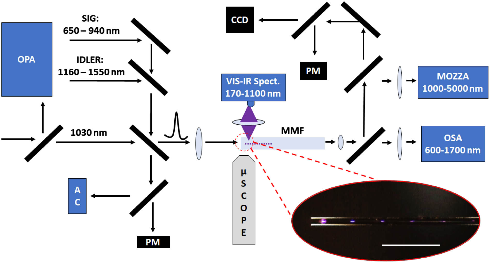
Fig. 1. Experimental setup to characterize the NL of MMFs. In the inset, we show a microscope image of the scattered PL in correspondence of the self-imaging points of a 50/125 GIF. The white scale bar is 1 mm long.

Fig. 2. (a) Dependence of output pulse energy versus the input energy, at λ=1030  nm (normal dispersion) or λ=1550  nm (anomalous dispersion) for 1 m of GIF. The dashed line represents the 100% normalized transmission curve. (b) Pump spectra. (c) and (d) Output spectral evolution for different input peak powers at 1030 nm (c) or 1550 nm (d), respectively. The corresponding input pulse duration is 174 fs and 61 fs, respectively, while the laser repetition rate is 100 kHz. The visible range of the output spectra was collected by means of the same spectrometer that was used for characterizing PL.

Fig. 3. Output average power versus the laser repetition rate, for 0.8 MW (linear loss regime) or 1.9 MW (NL regime) of input power. The laser wavelength and pulse duration were set to 1030 nm and 174 fs, respectively. The inset shows a microscope image of the input tip of a 50/125 GIF, after picosecond laser pulses with power right above the breakdown threshold were injected for a few minutes.

Fig. 4. (a) and (b) Microscope images of the (a) SIF and (b) GIF when the defects’ PL is excited by MPA of a 2 MW input peak power laser beam. (c), (d) Same as (a), (b), with the room light switched off. The white bar is 1 mm long. (e) Comparison between the two MMFs normalized transmission, versus input pulse energy, for a pulse duration of 174 fs (circle markers, solid lines) or 7.9 ps (square markers, dashed lines).

Fig. 5. (a) Side-scattered spectra for different source wavelengths at Pp=2.5  MW of input peak power. (b) Input spectra at different wavelengths. (c) Log–log plot of the Ge-ODC PL intensity IPL versus Pp. The intensities are calculated as the integral of the corresponding peaks in the output spectrum. In the legend, the number in parenthesis denotes the calculated NPL. (d) Fiber NL for different source wavelengths. (e) Comparison between the fiber transmission at Pp=4  MW and NPL versus source wavelength.

Fig. 6. (a) Side-scattering spectrum, obtained when varying the slit position. (b) Integral of the spectral peaks in (a). Solid lines are a guide for the eye. (c) Cutback experiment from 10 cm to 1.5 cm of fiber length. The Pp value was varied by changing the input pulse duration between 7.9 ps and 174 fs, while keeping the pulse energy unchanged. (d) PL intensity variation along with Pp. Images from the top to the bottom correspond to Pp=1.62, 1.89, 2.16, and 2.43 MW, respectively.

Fig. 7. (a) Detail of the beam size minimum, for different values of Pp. (b) Beam size oscillation along the propagation distance, for Pp=2  MW. (c) Evolution of beam intensity (normalized to its maximum value) and transmission along the first 5 mm of GIF, as obtained from the N-photon absorption model in Eq. (3) with N=3 and α3=10−31  m3/W2.

Fig. 8. Fit of the cutback experimental data in Fig. 6(c) with the model in Eq. (3). The fit parameters are N=3.008 and αN=2.415×10−33. Panels (α−η) provide details of the fit at different distances z, taken at points shown by the central panel.