
Yanan Han, Shuiying Xiang, Zhenxing Ren, Chentao Fu, Aijun Wen, Yue Hao, "Delay-weight plasticity-based supervised learning in optical spiking neural networks," Photonics Res. 9, B119 (2021)
- Photonics Research
- Vol. 9, Issue 4, B119 (2021)
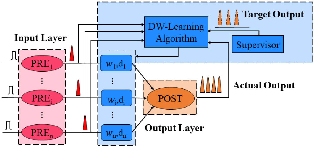
Fig. 1. Schematic diagram of DW-based learning in a single-layer photonic SNN.
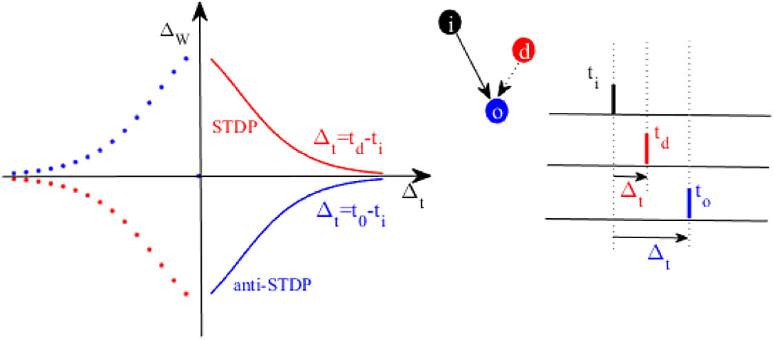
Fig. 2. Schematic illustration of the ReSuMe incorporated with optical STDP rule. i d o
Fig. 3. (a1) and (b1) Input pattern and output pattern before delay adjustment. (a2) and (b2) After 7 training epochs.
Fig. 4. Comparison of the learning capability of a single neuron based on (a) weight-based ReSuMe and (b) DW-ReSuMe. The value of SSD after the 50th, 100th, and 300th training epoch is presented for different t i η ω ω 0 ω 0 η ω n = 1 t d = 8 ns
Fig. 5. (a1) Carrier density of the POST after training and (b1) the evolution of output spikes based on the DW-ReSuMe; (a2) and (b2) those based on ReSuMe. The black solid line is n a P .
Fig. 6. Evolution of (a1) synaptic weights ω i d i
Fig. 7. Learning spike sequences with ununiformed ISI. (a1) and (b1) The evolution of output spikes for spike sequence [10 ns, 12 ns, 14 ns, 18 ns, 20 ns, 22 ns, 24 ns, 26 ns, 29 ns] and [10 ns, 11 ns, 13 ns, 14.5 ns, 17 ns, 21 ns, 23 ns, 25.5 ns, 27 ns], respectively. (a2) and (b2) The evolution for the corresponding distance.
Fig. 8. (a) Training accuracy and (b) testing accuracy varying with training epochs for weight-based ReSuMe (blue solid line) and DW-ReSuMe (red solid line). T d = 1 ns T ω = 4 ns
Fig. 9. Illustration of classification results for (a) training data set and (b) testing data set. The orange cycles denote target spiking time, the blue squares represent the actual spiking time, and misclassified samples are highlighted in bright blue.
Fig. 10. Testing accuracy as a function of (a) weight learning window T ω T d
Fig. 11. (a) Training accuracy and (b) testing accuracy varying with training epochs based on DW-ReSuMe (red solid line) and ReSuMe (blue solid line), respectively. T d = 4 ns T ω = 5 ns
Fig. 12. (a1) Training accuracy and (a2) testing accuracy for the Iris data set after 60 training epochs with different initial delay d 0
Fig. 13. Learning accuracy of the breast cancer data set based on DW-ReSuMe with different cases of η d η d η d T d = 4 ns T ω = 5 ns


Set citation alerts for the article
Please enter your email address

© Copyright 2018-2021 | Chinese Laser Press. All Rights Reserved 沪ICP备15018463号-20