• Matter and Radiation at Extremes
  • Vol. 7, Issue 4, 046901 (2022)
A. F. A. Bott1、2、a), L. Chen1, P. Tzeferacos1、3、4, C. A. J. Palmer5, A. R. Bell1, R. Bingham6、7, A. Birkel8, D. H. Froula3、4, J. Katz4, M. W. Kunz2, C.-K. Li8, H-S. Park9, R. Petrasso8, J. S. Ross9, B. Reville0, D. Ryu0, F. H. Séguin8, T. G. White0, A. A. Schekochihin1, D. Q. Lamb0, and G. Gregori0、1
Author Affiliations
  • 0Department of Astronomy and Astrophysics, University of Chicago, Chicago, Illinois 60637, USA
  • 0Department of Physics, School of Natural Sciences, UNIST, Ulsan, South Korea
  • 0Department of Physics, University of Nevada, Reno, Nevada 89557, USA
  • 0Max-Planck-Institut für Kernphysik, Heidelberg, Germany
  • 1Department of Physics, University of Oxford, Oxford, United Kingdom
  • 2Department of Astrophysical Sciences, University of Princeton, Princeton, New Jersey 08544, USA
  • 3Department of Physics and Astronomy, University of Rochester, Rochester, New York 14627, USA
  • 4Laboratory for Laser Energetics, University of Rochester, Rochester, New York 14623, USA
  • 5School of Mathematics and Physics, Queens University Belfast, Belfast, United Kingdom
  • 6Rutherford Appleton Laboratory, Chilton, Didcot, United Kingdom
  • 7Department of Physics, University of Strathclyde, Glasgow, United Kingdom
  • 8Massachusetts Institute of Technology, Cambridge, Massachusetts 02139, USA
  • 9Lawrence Livermore National Laboratory, Livermore, California 94550, USA
  • show less
    DOI: 10.1063/5.0084345 Cite this Article
    A. F. A. Bott, L. Chen, P. Tzeferacos, C. A. J. Palmer, A. R. Bell, R. Bingham, A. Birkel, D. H. Froula, J. Katz, M. W. Kunz, C.-K. Li, H-S. Park, R. Petrasso, J. S. Ross, B. Reville, D. Ryu, F. H. Séguin, T. G. White, A. A. Schekochihin, D. Q. Lamb, G. Gregori. Insensitivity of a turbulent laser-plasma dynamo to initial conditions[J]. Matter and Radiation at Extremes, 2022, 7(4): 046901 Copy Citation Text show less
    Schematic of the experimental setup. Twenty beams of the OMEGA laser deliver a total of 10 kJ of 351 nm-wavelength laser-light energy over 10 ns to an 800 μm-diameter focal spot on two CH plastic foils (5 kJ/foil). The foils have the same design used in a previous experiment at the Omega Laser Facility.38 The primary foils have thicknesses of 50 µm and are attached to annular washers with an outer diameter of 3 mm, a central hole with a diameter of 400 µm, and a thickness of 230 µm. The grids used on the target are also the same. They have 300 μm-square holes and 100 μm wires (periodicity L ≈ 400 µm), and are asymmetric, with the midpoints of the holes in one grid always facing the midpoints of the wire intersections in the other. The magneto-inertial fusion electrical discharge system (MIFEDS) is operated at 19 kV, with the maximum voltage coinciding with drive-beam initiation. The morphology of the initial magnetic field is indicated in light blue. The location of the interaction-region plasma is indicated, as is the path of the Thomson scattering (TS) probe beam (in yellow). The central axis of the proton-radiography beam and the area probed by it are indicated in red.
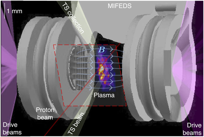
    Fig. 1. Schematic of the experimental setup. Twenty beams of the OMEGA laser deliver a total of 10 kJ of 351 nm-wavelength laser-light energy over 10 ns to an 800 μm-diameter focal spot on two CH plastic foils (5 kJ/foil). The foils have the same design used in a previous experiment at the Omega Laser Facility.38 The primary foils have thicknesses of 50 µm and are attached to annular washers with an outer diameter of 3 mm, a central hole with a diameter of 400 µm, and a thickness of 230 µm. The grids used on the target are also the same. They have 300 μm-square holes and 100 μm wires (periodicity L ≈ 400 µm), and are asymmetric, with the midpoints of the holes in one grid always facing the midpoints of the wire intersections in the other. The magneto-inertial fusion electrical discharge system (MIFEDS) is operated at 19 kV, with the maximum voltage coinciding with drive-beam initiation. The morphology of the initial magnetic field is indicated in light blue. The location of the interaction-region plasma is indicated, as is the path of the Thomson scattering (TS) probe beam (in yellow). The central axis of the proton-radiography beam and the area probed by it are indicated in red.
    XRFC images of soft x rays emitted by the turbulent plasma in both the presence (left) and absence (right) of the MIFEDS. The top row (22.5 ns after the start of the drive-beam) employed a 100 V bias on the XRFC, whereas all other (post-collision) images used 350 V (the former having 32× sensitivity). The resolution of the images, which is set by the pinhole size and the MCP response, was ∼50 µm. For reference, a projection of the target is shown on each image as a gray shade.
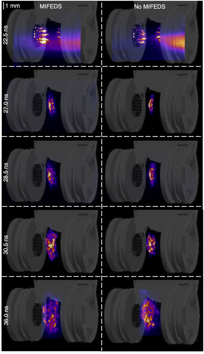
    Fig. 2. XRFC images of soft x rays emitted by the turbulent plasma in both the presence (left) and absence (right) of the MIFEDS. The top row (22.5 ns after the start of the drive-beam) employed a 100 V bias on the XRFC, whereas all other (post-collision) images used 350 V (the former having 32× sensitivity). The resolution of the images, which is set by the pinhole size and the MCP response, was ∼50 µm. For reference, a projection of the target is shown on each image as a gray shade.
    Maps of fluctuations in the detected x-ray intensity relative to a smooth mean intensity profile. The gray shaded regions denote the intervals over which the mean x-ray intensity profile is averaged when determining li (see text).
    Fig. 3. Maps of fluctuations in the detected x-ray intensity relative to a smooth mean intensity profile. The gray shaded regions denote the intervals over which the mean x-ray intensity profile is averaged when determining li (see text).
    Quantitative analysis of x-ray images. (a) Evolution of the transverse width of the interaction region li over time in the presence (blue squares) and absence (red crosses) of MIFEDS. (b) Evolution over time of the inferred rms magnitude of density fluctuations in the plasma. (c) Evolution over time of the inferred integral length ln of density fluctuations in the plasma.
    Fig. 4. Quantitative analysis of x-ray images. (a) Evolution of the transverse width of the interaction region li over time in the presence (blue squares) and absence (red crosses) of MIFEDS. (b) Evolution over time of the inferred rms magnitude of density fluctuations in the plasma. (c) Evolution over time of the inferred integral length ln of density fluctuations in the plasma.
    Inferred spectra of relative x-ray density and velocity fluctuations in the plasma at four different times in the presence and absence of the MIFEDS magnetic field.
    Fig. 5. Inferred spectra of relative x-ray density and velocity fluctuations in the plasma at four different times in the presence and absence of the MIFEDS magnetic field.
    Thomson-scattering data and fitting. (a) Time-resolved EPW spectral features obtained in the experiment. The absolute magnitude of the signals was normalized to the same value in each image. For the no-MIFEDS experiment (far left panel), the spectrometer used to detect the EPW spectral feature gave an erroneous output for a 200 ps interval centered at 24.0 ns; this output is masked. (b) Plot of the experimental signal (solid red line) obtained from the raw data shown in the far-left panel of (a) by averaging over a 100 ps interval centered at 24.15 ns (viz., the interval indicated by the white translucent region). The blue dot-dashed line indicates the fit to the background signal that we subtract prior to constructing a best-fit model to the EPW spectral feature. (c) Plot of the experimental signal (with the background subtracted) obtained from the raw data shown in the mid-left panel of (a) by averaging over an 100 ps interval centered at 24.15 ns, along with three possible spectral fits with different mean electron number densities: n̄e=ne,fit=4.3×1019cm−3 (solid blue line), n̄e=0.85ne,fit=3.6×1019cm−3 (dotted blue line), and n̄e=1.15ne,fit=3.6×1019cm−3 (dashed blue line). The assumed electron temperature was Te = 550 eV. (d) Same as (c) but at 26.15 ns and for three possible spectral fits with different electron temperatures (and mean electron number densities): n̄e=ne,fit=7.9,×,1019cm−3 and Te = Te,fit = 380 eV (solid blue line); n̄e=1.1ne,fit=8.7×1019cm−3 and Te = 0.5Te,fit = 190 eV (dotted blue line); and n̄e=0.9ne,fit=7.1×1019cm−3 and Te = 1.5Te,fit = 570 eV (dashed blue line). A Gaussian spread of densities with Δne/n̄e=0.25 was assumed. (e) Same as (c), but at 28.15 ns and for two possible spectral fits (both with n̄e=ne,fit=8.8×1019cm−3 and Te = Te,fit = 380 eV): Δne/n̄e=0.25 (solid blue line) and Δne/n̄e=0 (dotted-dashed blue line).
    Fig. 6. Thomson-scattering data and fitting. (a) Time-resolved EPW spectral features obtained in the experiment. The absolute magnitude of the signals was normalized to the same value in each image. For the no-MIFEDS experiment (far left panel), the spectrometer used to detect the EPW spectral feature gave an erroneous output for a 200 ps interval centered at 24.0 ns; this output is masked. (b) Plot of the experimental signal (solid red line) obtained from the raw data shown in the far-left panel of (a) by averaging over a 100 ps interval centered at 24.15 ns (viz., the interval indicated by the white translucent region). The blue dot-dashed line indicates the fit to the background signal that we subtract prior to constructing a best-fit model to the EPW spectral feature. (c) Plot of the experimental signal (with the background subtracted) obtained from the raw data shown in the mid-left panel of (a) by averaging over an 100 ps interval centered at 24.15 ns, along with three possible spectral fits with different mean electron number densities: n̄e=ne,fit=4.3×1019cm3 (solid blue line), n̄e=0.85ne,fit=3.6×1019cm3 (dotted blue line), and n̄e=1.15ne,fit=3.6×1019cm3 (dashed blue line). The assumed electron temperature was Te = 550 eV. (d) Same as (c) but at 26.15 ns and for three possible spectral fits with different electron temperatures (and mean electron number densities): n̄e=ne,fit=7.9,×,1019cm3 and Te = Te,fit = 380 eV (solid blue line); n̄e=1.1ne,fit=8.7×1019cm3 and Te = 0.5Te,fit = 190 eV (dotted blue line); and n̄e=0.9ne,fit=7.1×1019cm3 and Te = 1.5Te,fit = 570 eV (dashed blue line). A Gaussian spread of densities with Δne/n̄e=0.25 was assumed. (e) Same as (c), but at 28.15 ns and for two possible spectral fits (both with n̄e=ne,fit=8.8×1019cm3 and Te = Te,fit = 380 eV): Δne/n̄e=0.25 (solid blue line) and Δne/n̄e=0 (dotted-dashed blue line).
    Thomson-scattering derived measurements of the physical state of the plasma showing the evolution of the electron number density and temperature in the presence and absence of the MIFEDS magnetic field around and just after collision, as inferred from spectral fits.
    Fig. 7. Thomson-scattering derived measurements of the physical state of the plasma showing the evolution of the electron number density and temperature in the presence and absence of the MIFEDS magnetic field around and just after collision, as inferred from spectral fits.
    Calibration measurement of the MIFEDS magnetic field with proton radiography. Left: 15.0 MeV proton radiograph of the target in the absence of any drive beams but with MIFEDS on. The axes of the image, which has a 28× magnification, are rescaled so that lengths are directly comparable with the plasma scale. The reported pixel counts are normalized to their mean value (∼60 protons/pixel) in a 0.1 × 0.1 cm2 square whose midpoint is at the center of each image. Right: 3.3 MeV proton radiograph for the same setup. In both panels, the red line marks the apparent boundary of the 15.0 MeV proton beam, while the gold line marks the apparent boundary of the 3.3 MeV proton beam. The solid purple line marks the boundary of both proton beams in the absence of any magnetic fields. It was inferred from the relative displacement of the apparent boundary of the 15.0 and 3.3 MeV beams. The short-dashed, medium-dashed, and long-dashed lines denote the observed boundary of the 15.0 MeV proton beams at 25.2, 31.2, and 38.7 ns, respectively, in the no-MIFEDS experiments. In these images, the line of centers is vertical and the targets and grids lie at the top and the bottom of it.
    Fig. 8. Calibration measurement of the MIFEDS magnetic field with proton radiography. Left: 15.0 MeV proton radiograph of the target in the absence of any drive beams but with MIFEDS on. The axes of the image, which has a 28× magnification, are rescaled so that lengths are directly comparable with the plasma scale. The reported pixel counts are normalized to their mean value (∼60 protons/pixel) in a 0.1 × 0.1 cm2 square whose midpoint is at the center of each image. Right: 3.3 MeV proton radiograph for the same setup. In both panels, the red line marks the apparent boundary of the 15.0 MeV proton beam, while the gold line marks the apparent boundary of the 3.3 MeV proton beam. The solid purple line marks the boundary of both proton beams in the absence of any magnetic fields. It was inferred from the relative displacement of the apparent boundary of the 15.0 and 3.3 MeV beams. The short-dashed, medium-dashed, and long-dashed lines denote the observed boundary of the 15.0 MeV proton beams at 25.2, 31.2, and 38.7 ns, respectively, in the no-MIFEDS experiments. In these images, the line of centers is vertical and the targets and grids lie at the top and the bottom of it.
    Proton radiography measurements of magnetic fields at collision. Left column: 15.0 MeV-proton radiographs in the presence and absence of the MIFEDS at 25.2 ns (at a time close to the collision of the plasma jets). The pixel counts of each image are normalized to their mean value (∼60 protons/pixel) in a 0.1 × 0.1 cm2 square whose midpoint is at the center of each image. In these images, the line of centers is vertical and the targets and grids lie at the top and bottom of it. The interaction region is offset by ∼0.05 cm leftward in the MIFEDS image due to the effect of the large-scale MIFEDS magnetic field. Right column: Magnitude of the “small-scale” components of the path-integrated magnetic field that is perpendicular to the trajectory of the proton radiography beam. In each case, we determine this quantity over a region that is approximately coincident with the location of the interaction-region plasma, and only show those fluctuations in the path-integrated magnetic field whose characteristic scale is smaller than the characteristic size of the region analyzed. When the MIFEDS is on, we recover a large-scale path-integrated magnetic field in addition to the small-scale path-integrated field that causes the deflection of protons leftward. To enable a direct comparison, this field is not shown, and the positioning of the small-scale path-integrated field in these cases is adjusted to take this deflection into account.
    Fig. 9. Proton radiography measurements of magnetic fields at collision. Left column: 15.0 MeV-proton radiographs in the presence and absence of the MIFEDS at 25.2 ns (at a time close to the collision of the plasma jets). The pixel counts of each image are normalized to their mean value (∼60 protons/pixel) in a 0.1 × 0.1 cm2 square whose midpoint is at the center of each image. In these images, the line of centers is vertical and the targets and grids lie at the top and bottom of it. The interaction region is offset by ∼0.05 cm leftward in the MIFEDS image due to the effect of the large-scale MIFEDS magnetic field. Right column: Magnitude of the “small-scale” components of the path-integrated magnetic field that is perpendicular to the trajectory of the proton radiography beam. In each case, we determine this quantity over a region that is approximately coincident with the location of the interaction-region plasma, and only show those fluctuations in the path-integrated magnetic field whose characteristic scale is smaller than the characteristic size of the region analyzed. When the MIFEDS is on, we recover a large-scale path-integrated magnetic field in addition to the small-scale path-integrated field that causes the deflection of protons leftward. To enable a direct comparison, this field is not shown, and the positioning of the small-scale path-integrated field in these cases is adjusted to take this deflection into account.
    Proton radiography measurements of magnetic fields post-collision. Left column: 15.0 MeV proton radiographs in the presence and absence of the MIFEDS ∼6 ns after collision. Each image is normalized to its mean value (∼60 protons/pixel) in a 0.1 × 0.1 cm2 area in the center of each image. In these images, the line of centers is vertical and the targets and grids lie at the top and bottom of it. The interaction region is offset by ∼0.05 cm leftward in the MIFEDS image due to the effect of the large-scale MIFEDS magnetic field. The long horizontal feature in the MIFEDS image lies to the right of the interaction region (see text). Right column: Magnitude of the small-scale components of the (perpendicular) path-integrated magnetic field.
    Fig. 10. Proton radiography measurements of magnetic fields post-collision. Left column: 15.0 MeV proton radiographs in the presence and absence of the MIFEDS ∼6 ns after collision. Each image is normalized to its mean value (∼60 protons/pixel) in a 0.1 × 0.1 cm2 area in the center of each image. In these images, the line of centers is vertical and the targets and grids lie at the top and bottom of it. The interaction region is offset by ∼0.05 cm leftward in the MIFEDS image due to the effect of the large-scale MIFEDS magnetic field. The long horizontal feature in the MIFEDS image lies to the right of the interaction region (see text). Right column: Magnitude of the small-scale components of the (perpendicular) path-integrated magnetic field.
    Proton radiography measurements of magnetic fields at late times. Left column: 15.0 MeV proton radiographs in the presence and absence of the MIFEDS 13.5 ns after collision. The proton flux is detected using a CR-39 detector stack. The pixel counts of each image are normalized to their mean value (∼60 protons/pixel) in a 0.1 × 0.1 cm2 square whose midpoint is at the center of each image. In these images, the line of centers is vertical and the targets and grids lie at the top and bottom of it. The interaction region is offset by ∼0.05 cm leftward in the MIFEDS image due to the effect of the large-scale MIFEDS magnetic field. The long horizontal feature in the MIFEDS image lies to the right of the interaction region (see text). Right column: Magnitude of the small-scale components of the (perpendicular) path-integrated magnetic field.
    Fig. 11. Proton radiography measurements of magnetic fields at late times. Left column: 15.0 MeV proton radiographs in the presence and absence of the MIFEDS 13.5 ns after collision. The proton flux is detected using a CR-39 detector stack. The pixel counts of each image are normalized to their mean value (∼60 protons/pixel) in a 0.1 × 0.1 cm2 square whose midpoint is at the center of each image. In these images, the line of centers is vertical and the targets and grids lie at the top and bottom of it. The interaction region is offset by ∼0.05 cm leftward in the MIFEDS image due to the effect of the large-scale MIFEDS magnetic field. The long horizontal feature in the MIFEDS image lies to the right of the interaction region (see text). Right column: Magnitude of the small-scale components of the (perpendicular) path-integrated magnetic field.
    Proton radiography measurements of magnetic-energy spectra. Spectra obtained from no-MIFEDS experiments are shown in red, and those from MIFEDS experiments in blue. The nominal limit on the resolution due to the finite size of the proton source is indicated on each plot. However, the actual resolution scale is observed to be a few times larger than indicated due to a systematic blurring of the proton-radiography data that stems from self-intersection of the proton beam prior to its detection. The self-intersection is caused by small-scale stochastic magnetic fields in the plasma.40,60 The uncertainty of the measurement of the spectra was estimated by assuming that the interaction-region plasma is homogeneous, and then treating the left- and right-hand sides of the interaction region as independent samples. Left: 31.2 ns after collision. Right: 38.7 ns after collision.
    Fig. 12. Proton radiography measurements of magnetic-energy spectra. Spectra obtained from no-MIFEDS experiments are shown in red, and those from MIFEDS experiments in blue. The nominal limit on the resolution due to the finite size of the proton source is indicated on each plot. However, the actual resolution scale is observed to be a few times larger than indicated due to a systematic blurring of the proton-radiography data that stems from self-intersection of the proton beam prior to its detection. The self-intersection is caused by small-scale stochastic magnetic fields in the plasma.40,60 The uncertainty of the measurement of the spectra was estimated by assuming that the interaction-region plasma is homogeneous, and then treating the left- and right-hand sides of the interaction region as independent samples. Left: 31.2 ns after collision. Right: 38.7 ns after collision.
    A. F. A. Bott, L. Chen, P. Tzeferacos, C. A. J. Palmer, A. R. Bell, R. Bingham, A. Birkel, D. H. Froula, J. Katz, M. W. Kunz, C.-K. Li, H-S. Park, R. Petrasso, J. S. Ross, B. Reville, D. Ryu, F. H. Séguin, T. G. White, A. A. Schekochihin, D. Q. Lamb, G. Gregori. Insensitivity of a turbulent laser-plasma dynamo to initial conditions[J]. Matter and Radiation at Extremes, 2022, 7(4): 046901
    Download Citation