In high-power laser systems, such as NOVA, OMEGA, NIF, and SG-II, an auto-alignment system is very important because thousands of mirrors exist in hundreds of meters of beam lines^[1–6]. As high-power laser systems have developed from the MOPA-based to four-path concept, auto-alignment systems have been developed to meet the special requirements as laser systems have become more complicated. Moreover, the auto-alignment technique is continually developing as new equipment and tools are applied^[7–15]. The NIF is a typical four-path high-power laser system, which in its early years used a grating reference for alignment, and after years of development, a no-grating scheme has been applied^{[13, 14]}.

Auto-alignment processing loops always start with determining the current position and pointing angle of the beam, which requires a sensor in order to obtain the beam position displacement and pointing deviation angle from the reference (some type of mark). Second, the system must decide how much the mirror should be adjusted by means of analyzing the image acquired by the sensor. Then, the mirror is adjusted by driving motors for the corresponding steps, and the new beam position and pointing angle are verified by the sensor. This loop will stop when both the beam position and pointing angle meet the system requirements. Previous alignment methods typically required two optical sensors, one for the beam position and the other for its pointing angle. In certain situations, considering space or budget limitations, such as in outer space or vacuum chambers^[16], high temperatures or cryogenic environments, and high radiation situations, the sensor needs to be very small or lightweight. We propose a sensor with only one lens, one plate, and one camera, which improves on the previous methods by including a type of sensor with one camera^[17]. Because this method is so simple and stable, it can not only operate as a sensor, but also serve as an effective reference.

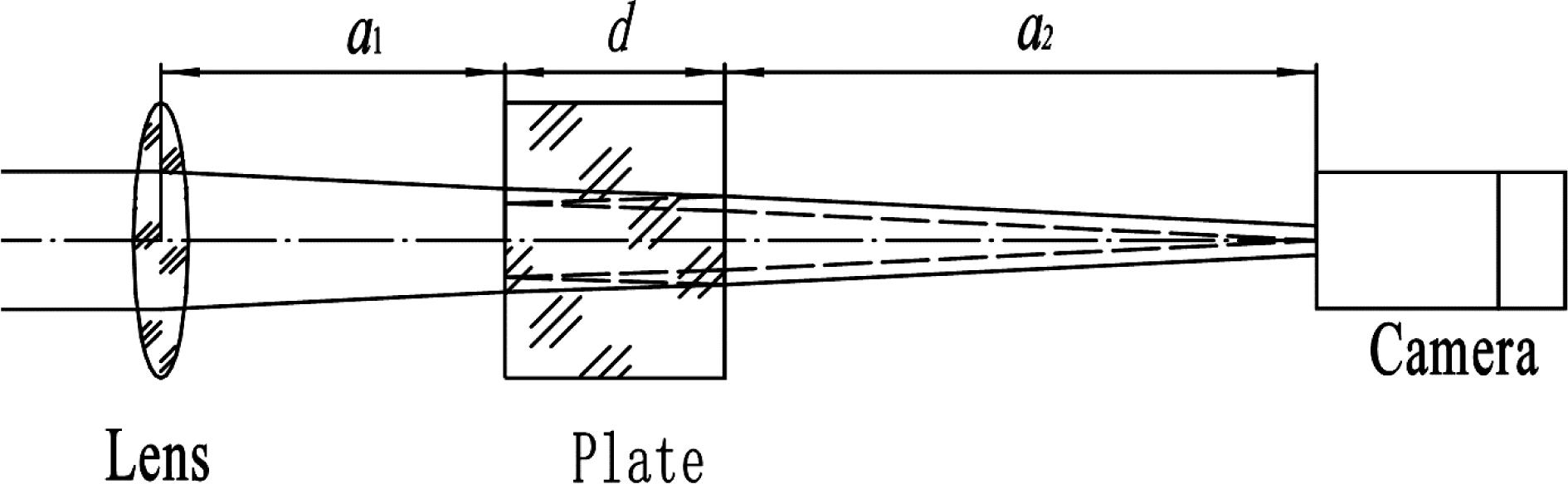
The single lens alignment sensor is designed on the basis of the ‘ghost image concept’, and consists of a lens, parallel plate, and camera (see Figure 1). The normals of the plate and camera surfaces should be parallel to the lens axis. When placing the camera on the focal plane of the second-order ghost image of the input beam led by the plate, the camera will detect both the beam profile and focal spot in one image. With a special coat on the plate, the ‘ghost’ is significantly brightened, and the brightness is sufficiently strong compared to that of the beam profile. In comparison with the two-sensor auto-alignment method, we refer to the beam profile image as near-field (or more accurately, quasi-near-field), and the ghost image as far-field.

Based on the matrix optics theory, we analyze the sensor operation. The transfer array from the lens to the camera for the original beam should be $$\begin{eqnarray}\displaystyle \left[\begin{array}{@{}cc@{}}\displaystyle 1-\frac{a_{1}+a_{2}}{f}-\frac{d}{fn} & \displaystyle a_{1}+a_{2}+\frac{d}{n}\\ \displaystyle -\frac{1}{f} & 1\end{array}\right], & & \displaystyle\end{eqnarray}$$(1) where $a_{1}$ is the distance from the lens to the plate’s front surface, $a_{2}$ is the distance from the camera to the plate’s rear surface, $d$ is the plate thickness, $n$ is the plate refractivity, and $f$ is the lens focus length.

Furthermore, the transfer array of the ghost beam should be $$\begin{eqnarray}\displaystyle \left[\begin{array}{@{}cc@{}}\displaystyle 1-\frac{a_{1}+a_{2}}{f}-\frac{3d}{fn} & \displaystyle a_{1}+a_{2}+\frac{3d}{n}\\ \displaystyle -\frac{1}{f} & 1\\ \end{array}\right]. & & \displaystyle\end{eqnarray}$$(2) Because the camera is located at the focal spot of the lens, the sensor parameters should satisfy the following correlation: $$\begin{eqnarray}\displaystyle a_{2}=f-a_{1}-3d/n. & & \displaystyle\end{eqnarray}$$(3) In this case, the transfer array should be rewritten as $$\begin{eqnarray}\displaystyle \left[\begin{array}{@{}cc@{}}2d/fn & f-2d/n\\ -1/f & 1\end{array}\right], & & \displaystyle\end{eqnarray}$$(4) and $$\begin{eqnarray}\displaystyle \left[\begin{array}{@{}cc@{}}0 & f\\ -1/f & 1\end{array}\right]. & & \displaystyle\end{eqnarray}$$(5) These are functions of $f$, $n$, $d$, which means that the plate position ($a_{1}$) does not contribute anything to the transfer array.

Taking the lens center and axis as the alignment reference, the optics array of the input laser beam should be written as $$\begin{eqnarray}\displaystyle A_{\text{in}}=\left[\begin{array}{@{}cc@{}}r_{X} & r_{Y}\\ \unicode[STIX]{x1D703}_{X} & \unicode[STIX]{x1D703}_{Y}\end{array}\right], & & \displaystyle\end{eqnarray}$$(6) where $r_{X}$ and $r_{Y}$ are horizontal and vertical displacement, respectively, of the laser beam center on the input surface of the lens from the lens center, while $\unicode[STIX]{x1D703}_{X}$ and $\unicode[STIX]{x1D703}_{Y}$ are the azimuth and altitude deviation, respectively, of the beam pointing direction from the lens axis. Then, we can determine the near-field and far-field positions on the camera: $$\begin{eqnarray}\displaystyle \left\{\begin{array}{@{}l@{}}x_{\text{FF}}=f\unicode[STIX]{x1D703}_{X}\\ x_{\text{NF}}=2dr_{X}/fn+f\unicode[STIX]{x1D703}_{X}-2d\unicode[STIX]{x1D703}_{X}/n,\end{array}\right. & & \displaystyle\end{eqnarray}$$(7)$$\begin{eqnarray}\displaystyle \left\{\begin{array}{@{}l@{}}y_{\text{FF}}=f\unicode[STIX]{x1D703}_{Y}\\ y_{\text{NF}}=2dr_{Y}/fn+f\unicode[STIX]{x1D703}_{Y}-2d\unicode[STIX]{x1D703}_{Y}/n,\end{array}\right. & & \displaystyle\end{eqnarray}$$(8) where ($x_{\text{FF}}$, $y_{\text{FF}}$) is the far-field center on the camera, and ($x_{\text{NF}}$, $y_{\text{NF}}$) is the near-field center on the camera.

Camera image acquisition provides an image including both the near-field and far-field, and we can determine the input beam position and pointing angle from the image as follows: $$\begin{eqnarray}\displaystyle \left\{\begin{array}{@{}l@{}}r_{X}=x_{\text{FF}}+(x_{\text{NF}}-x_{\text{FF}})fn/2d,\\ \unicode[STIX]{x1D703}_{X}=x_{\text{FF}}/f,\end{array}\right. & & \displaystyle\end{eqnarray}$$(9) and $$\begin{eqnarray}\displaystyle \left\{\begin{array}{@{}l@{}}r_{Y}=y_{\text{FF}}+(y_{\text{NF}}-y_{\text{FF}})fn/2d,\\ \unicode[STIX]{x1D703}_{Y}=y_{\text{FF}}/f.\end{array}\right. & & \displaystyle\end{eqnarray}$$(10) If the sensor is installed as a reference, the target position can be described as $$\begin{eqnarray}\displaystyle A_{\text{ref}}=\left[\begin{array}{@{}cc@{}}0 & 0\\ 0 & 0\end{array}\right]. & & \displaystyle\end{eqnarray}$$(11) In this case, suppose that the camera sensor center is located accurately on the lens axis and the surfaces of the plate are parallel, then the far-field and near-field should be in the center of the image acquired by the camera. The mirrors are driven for alignment until the far-field and near-field centers move to the image center with an acceptable error.

In order to perform alignment of a beam path, we need to know the beam aperture ($A$), near-field tolerance (maximum deviation from reference $D_{c}$), and position alignment accuracy requirement ($R_{\text{NF}}$), while for the pointing angle, we need to know the far-field tolerance ($\unicode[STIX]{x1D703}_{c}$) and pointing angle alignment accuracy requirement ($R_{\text{FF}}$). The reference and sensor must meet all of the requirements, which need to be considered in order to determine the sensor parameters. When designing the sensor, there are certain basic rules for laser system beam alignment that should be obeyed.

The correlation between the sensor parameters and the alignment concerned specifications is analyzed in this section. As illustrated in Figure 1 and discussed above, the sensor parameters include the lens parameters (focal length $f$ and diameter $D$), plate parameters (thickness $d$, refractive index $n$, and reflectivity at front side $r_{1}$ and rear side $r_{2}$) and camera parameters (pixel size $R_{c}$ and sensor size $M$). Most of the time, optical systems are designed with axial symmetry; therefore, we simply discuss one dimension.

The near-field size on the camera is $$\begin{eqnarray}\displaystyle D_{\text{NF}}=2dA/f. & & \displaystyle\end{eqnarray}$$(12) By using the ideal divergence angle of the laser beam, the far-field spot size on the camera is $$\begin{eqnarray}\displaystyle D_{\text{FF}}=2.44f\unicode[STIX]{x1D706}/A. & & \displaystyle\end{eqnarray}$$(13) Considering the worst situation, the position and pointing angle limits add up at the same side of the lens axis, so the camera’s minimal size should be $$\begin{eqnarray}\displaystyle M_{\text{min}}=D_{c}+(f-2d/n)\unicode[STIX]{x1D703}_{c}+D_{\text{NF}}. & & \displaystyle\end{eqnarray}$$(14) In order to distinguish the far-field from near-field image, the far-field brightness should be 1 to 20 times that of the near-field. In most cases, as a result of optical system aberration, far-field brightness cannot be ideal; therefore, we estimate the focal spot size as $D_{\text{FF}}$. Based on the analysis, we get the correlation between the sensor parameters and the alignment concerned specifications, as is shown in Table 1.

As illustrated in Figure 2, a fiber output laser source @1053 nm is connected to a collimator, and the beam is expanded to ${\sim}\unicode[STIX]{x1D711}\;100~\text{mm}$. We use a serrated aperture to select a 33.4-mm diameter beam (calibrated at the lens front surface) for alignment (see Figure 3). The mirrors for alignment are 88 mm $\times$ 120 mm in size, operating at $45^{\circ }$. The sensor includes a lens ($f=954~\text{mm}@1053~\text{nm}$, $D=100~\text{mm}$), two pieces of plates (working together as one plate, using the plate 1 rear surface with a coating of reflectivity $r_{1}=10\%$ and front surface of plate 2 with a coating of reflectivity $r_{2}=10\%$, $n=1$, because the ghost is reflected between air gaps) and a camera ($R_{c}=8.3~\unicode[STIX]{x03BC}\text{m}/\text{pixel}$, size 782 pixel $\times$ 582 pixel).

The optics are roughly adjusted, as shown in Figure 2, and then the lens, plates and camera are adjusted, as described in Section 1. In the experiment, the single plate is replaced by two plates, simply because such a single plate with two sides of 10% coating is not often used in our laboratory, and needs to be processed specially for a certain designed alignment system, as described in Section 2. The alignment image captured by the sensor after adjustment is shown in Figure 4.

In order to prepare for the alignment task, the sensor will ‘teach’ the alignment mirrors how to carry out alignment work, or determine the response function of the alignment system: $$\begin{eqnarray}\displaystyle & & \displaystyle \left[\begin{array}{@{}c@{}}N_{X}\\ N_{Y}\\ F_{X}\\ F_{Y}\end{array}\right]\nonumber\\ \displaystyle & & \displaystyle \quad =\left[\begin{array}{@{}cccc@{}}r_{NX\_M1X} & r_{NX\_M1Y} & r_{NX\_M2X} & r_{NX\_M2Y}\\ r_{NY\_M1X} & r_{NY\_M1Y} & r_{NY\_M2X} & r_{NY\_M2Y}\\ r_{FX\_M1X} & r_{FX\_M1Y} & r_{FX\_M2X} & r_{FX\_M2Y}\\ r_{FY\_M1X} & r_{FY\_M1Y} & r_{FY\_M2X} & r_{FY\_M2Y}\end{array}\right]\left[\begin{array}{@{}c@{}}M_{1X}\\ M_{1Y}\\ M_{2X}\\ M_{2Y}\end{array}\right],\nonumber\\ \displaystyle & & \displaystyle\end{eqnarray}$$ (15) where $N_{X}$ ($N_{Y}$) is the near-field displacement on the camera (in pixels) in the horizontal (vertical) direction caused by mirror 1 and mirror 2 adjustment (counted in steps), while $F_{X}$ ($F_{Y}$) is the far-field displacement. Furthermore, $M_{1X}$ ($M_{1Y}$) represents the adjustment steps of mirror 1 in the horizontal (vertical) direction, while $M_{2X}$ ($M_{2Y}$) is the mirror 2 adjustment steps. When the mirror mount is designed to be orthogonal, Equation (15) can be $$\begin{eqnarray}\displaystyle & & \displaystyle \left[\begin{array}{@{}l@{}}N_{X}\\ N_{Y}\\ F_{X}\\ F_{Y}\end{array}\right]\nonumber\\ \displaystyle & & \displaystyle \quad =\left[\begin{array}{@{}cccc@{}}r_{NX\_M1X} & 0 & r_{NX\_M2X} & 0\\ 0 & r_{NY\_M1Y} & 0 & r_{NY\_M2Y}\\ r_{FX\_M1X} & 0 & r_{FX\_M2X} & 0\\ 0 & r_{FY\_M1Y} & 0 & r_{FY\_M2Y}\end{array}\right]\left[\begin{array}{@{}c@{}}M_{1X}\\ M_{1Y}\\ M_{2X}\\ M_{2Y}\end{array}\right].\nonumber\\ \displaystyle & & \displaystyle\end{eqnarray}$$ (16) In order to demonstrate the alignment loop by means of one-dimensional alignment, the horizontal direction or $x$-direction response function can be written as $$\begin{eqnarray}\displaystyle \left[\begin{array}{@{}c@{}}N_{X}\\ F_{X}\end{array}\right]=\left[\begin{array}{@{}cc@{}}r_{NX\_M1X} & r_{NX\_M2X}\\ r_{FX\_M1X} & r_{FX\_M2X}\end{array}\right]\left[\begin{array}{@{}c@{}}M_{1X}\\ M_{2X}\\ \end{array}\right]. & & \displaystyle\end{eqnarray}$$ (17) In order to determine the response array of the alignment system, we can check each array element by adjusting one by one the dimensions of each mirror (see Figure 5). Taking $r_{NX\_M1X}$ and $r_{FX\_M1X}$ as an example, first, we record an alignment image at the starting position, before the motor drives mirror 1 in the horizontal direction. Second, we drive mirror 1 in the horizontal direction by a certain number of steps each time (for example, 20 steps) and record the corresponding alignment image until sufficient images are obtained. Finally, we determine the center of the near-field and far-field for each image, and find the relationship ($r_{NX\_M1X}$ and $r_{FX\_M1X}$) between the mirror 1 adjustment steps and the near-field and far-field center positions (in pixels).

With each element of the response array, taking the average of different adjustment directions, we obtain the response function for the horizontal direction as follows: $$\begin{eqnarray}\displaystyle \left[\begin{array}{@{}c@{}}N_{X}\\ F_{X}\end{array}\right]=\left[\begin{array}{@{}cc@{}}-1.137 & 1.087\\ -1.157 & 1.125\end{array}\right]\left[\begin{array}{@{}c@{}}M_{1X}\\ M_{2X}\end{array}\right], & & \displaystyle\end{eqnarray}$$ (18) where $N_{X}$ and $N_{Y}$ are described in pixels, and $M_{1X}$ and $M_{2X}$ are described in steps.

After determining the response array, we can establish how to drive the mirrors when we obtain an alignment image (near-field and far-field center displacement from reference) by the sensor.

As the mirror mount experiences a motor empty back problem vertically, while working effectively in the horizontal direction, which is not the most important issue, we simply carry out horizontal alignment to test the sensor’s performance.

First, the image records the initial beam position of the beam (Figure 6(a)), and calculates the offset of the near-field center (232.8 pixels) and far-field center (246.1 pixels) from the reference (we take the camera center as the reference). According to Equation (18), the motor steps should be driven by $-$247 steps for mirror 1 and $-$473 steps for mirror 2 in the horizontal direction. However, we simply adjust three-quarter steps of these, namely $-$185 and $-$355 steps, for the purpose of reducing the out-of-step error, and then record the new position (Figure 6(b): 64.7 pixels for near-field and 67.6 pixels for far-field). Second, we calculate all of the remaining steps in the same manner, namely $-$32 steps for mirror 1 and $-$93 steps for mirror 2 in the horizontal direction. Following alignment image acquisition, we verify the result, which is only 1.9 pixels for near-field and 2.0 pixels for far-field deviation from the reference (Figure 6(c)).

The alignment accuracy is determined by both the controlling accuracy of the mirror mounts and sensor sensitivity. In the example discussed above, the mirror mount calibrated response is almost 1 pixel per step, which means that the controlling accuracy cannot be better than 1 pixel. Furthermore, the sensor cannot be better than 1 pixel, which is equal to $8.3~\unicode[STIX]{x03BC}\text{m}/954~\text{mm}=8.7~\unicode[STIX]{x03BC}\text{rad}$ for the pointing angle alignment, and $8.3~\unicode[STIX]{x03BC}\text{m}/1.7~\text{mm}=0.5\%$ or 0.16 mm for the 33.4 mm diameter beam for beam position alignment.

A single lens alignment sensor is designed on the basis of the ‘ghost image concept’. The working principle and performance analysis are demonstrated based on the theory of matrix optics. The design rules and alignment processing are defined, and an alignment example is carried out in order to demonstrate how the sensor works. The test results indicate that the sensor can operate effectively in the beam alignment process. The experimentally designed sensor performance is stable and can meet the alignment accuracy with approximately 0.5% for the position and $17.4~\unicode[STIX]{x03BC}\text{rad}$ for the pointing angle. Adjusting the focal length, plate thickness, and camera type can meet improved accuracy requirements.

References

[1] T. R. Boehly, D. L. Brown, R. S. Craxton, R. L. Keck, J. P. Knauer, J. H. Kelly, T. J. Kessler, S. A. Kumpan, S. J. Loucks, S. A. Letzring, F. J. Marshall, R. L. McCrory, S. F. B. Morse, W. Seka, J. M. Soures, C. P. Verdon. Opt. Commun., 1–6, 133(1997).
[2] C. A. Haynam, R. A. Sacks, P. J. Wegner, M. W. Bowers, S. N. Dixit, G. V. Erbert, G. M. Heestand, M. A. Henesian, M. R. Hermann, K. S. Jancaitis, K. R. Manes, C. D. Marshall, N. C. Mehta, J. Menapace, M. C. Nostrand, C. D. Orth, M. J. Shaw, S. B. Sutton, W. H. Williams, C. C. Widmayer, R. K. White, S. T. Yang, B. M. Van Wonterghem. Appl. Opt., 16, 46(2007).
[3] W. Zheng, X. Wei, Q. Zhu, F. Jing, D. Hu, J. Su, K. Zheng, X. Yuan, H. Zhou, W. Dai, W. Zhou, F. Wang, D. Xu, X. Xie, B. Feng, Z. Peng, L. Guo, Y. Chen, X. Zhang, L. Liu, D. Lin, Z. Dang, Y. Xiang, X. Deng. High Power Laser Sci. Eng., 4, e21(2016).
[4] G. Yanqi, C. Zhaodong, Y. Xuedong, M. Weixin, Z. Baoqiang, L. Zunqi. 11th Conference on Lasers and Electro-Optics Pacific Rim (CLEO-PR). Busan, South Korea, 1(2015).
[5] M. L. Andre. 2nd Annual International Conference on Solid State Lasers for Application to Inertial Confinement Fusion, 38(1996).
[6] L. Zunqi, W. Shiji, F. Dianyuan, Z. Jianqiang, Y. Yi, Z. Jian, C. Xijie, M. Weixin, Z. Dakui, S. Liqing, Z. Qingchun, X. Deyan, S. Weixing, C. Shaohe, C. Qinghao, P. Zengyun, L. Fengqiao, L. Liangyu, H. Guanlong, X. Zhenhua, T. Xianzhong. Chin. J. Lasers, 10B, 6(2001).
[7] E. S. Bliss, R. G. Ozarski, D. W. Myers, J. B. Richards, C. D. Swift, R. D. Boyd, R. E. Hugenberger, L. G. Seppala, J. Parker, E. H. Dryden. 9th Symposium on Engineering Problems of Fusion Research, 1242(1981).
[8] E. S. Bliss, S. J. Boege, R. D. Boyd, D. T. Davis, R. D. Demaret, M. Feldman, A. J. Gates, F. R. Holdener, C. F. Knopp, R. D. Kyker, C. W. Lauman, T. J. McCarville, J. L. Miller, V. J. Miller-Kamm, W. E. Rivera, J. T. Salmon, J. R. Severyn, S. K. Sheem, S. W. Thomas, C. E. Thompson, D. Y. Wang, M. F. Yoeman, R. A. Zacharias, C. Chocol, J. Hollis, D. Whitaker, J. Brucker, L. Bronisz, T. Sheridan. 3rd International Conference on Solid State Lasers for Application to Inertial Confinement Fusion, 285(1998).
[9] R. D. Boyd, E. S. Bliss, S. J. Boege, R. D. Demaret, M. Feldman, A. J. Gates, F. R. Holdener, J. Hollis, C. F. Knopp, T. J. McCarville, V. J. Miller-Kamm, W. E. Rivera, J. T. Salmon, J. R. Severyn, C. E. Thompson, D. Y. Wang, R. A. Zacharias. SPIE Conference on Optical Manufacturing and Testing III, 496(1999).
[10] Y.-Q. Gao, B.-Q. Zhu, D.-Z. Liu, X.-F. Liu, Z.-Q. Lin. Appl. Opt., 8, 48(2009).
[11] J. D. Lindl, E. I. Moses. Phys. Plasmas, 5, 18(2011).
[12] D. Liu, R. Xu, D. Fan. Chin. Opt. Lett., 2, 92(2004).
[13] S. C. Burkhart, E. Bliss, P. Di Nicola, D. Kalantar, R. Lowe-Webb, T. McCarville, D. Nelson, T. Salmon, T. Schindler, J. Villanueva, K. Wilhelmsen. Appl. Opt., 8, 50(2010).
[14] K. Wilhelmsen, A. Awwal, G. Brunton, S. Burkhart, D. McGuigan, V. M. Kamm, R. Leach, R. Lowe-Webb, R. Wilson. Fusion Engng Design, 12, 87(2012).
[15] R. Krappig, R. Schmitt. Conference on Photonic Instrumentation Engineering IV, 11(2017).
[16] W. Wu, L. Bi, K. Du, J. Zhang, H. Yang, H. Wang. High Power Laser Sci. Eng., 5, e9(2017).
[17] M. Charles.
Shun-Xing Tang, Ya-Jing Guo, Dai-Zhong Liu, Lin Yang, Xiu-Qing Jiang, Zeng-Yun Peng, Bao-Qiang Zhu. Single lens sensor and reference for auto-alignment[J]. High Power Laser Science and Engineering, 2018, 6(1): 010000e5
Download Citation