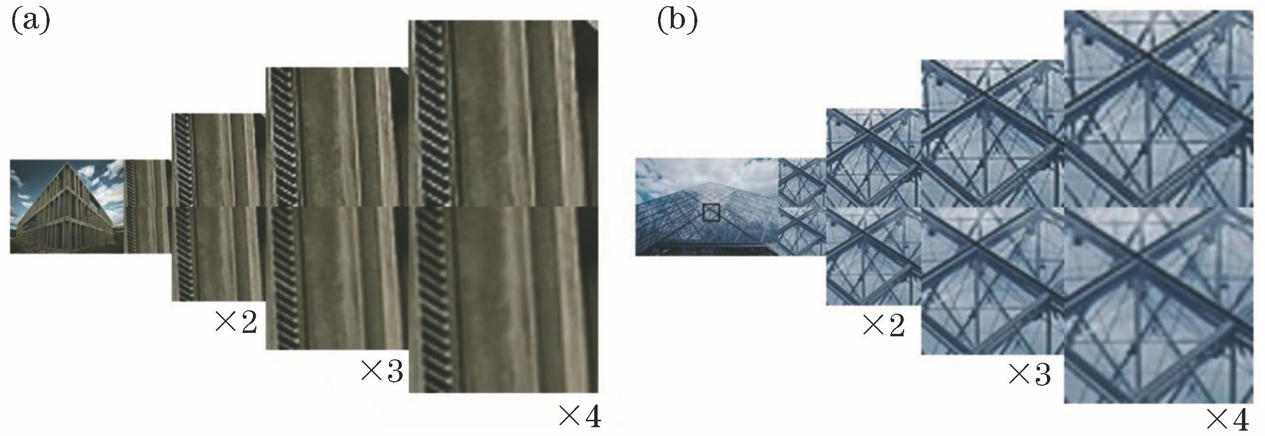
Fig. 1. DSSR (top) and LapSRN (bottom) algorithms deal with different images. (a) Images processed with different scale factors; (b) building edges result

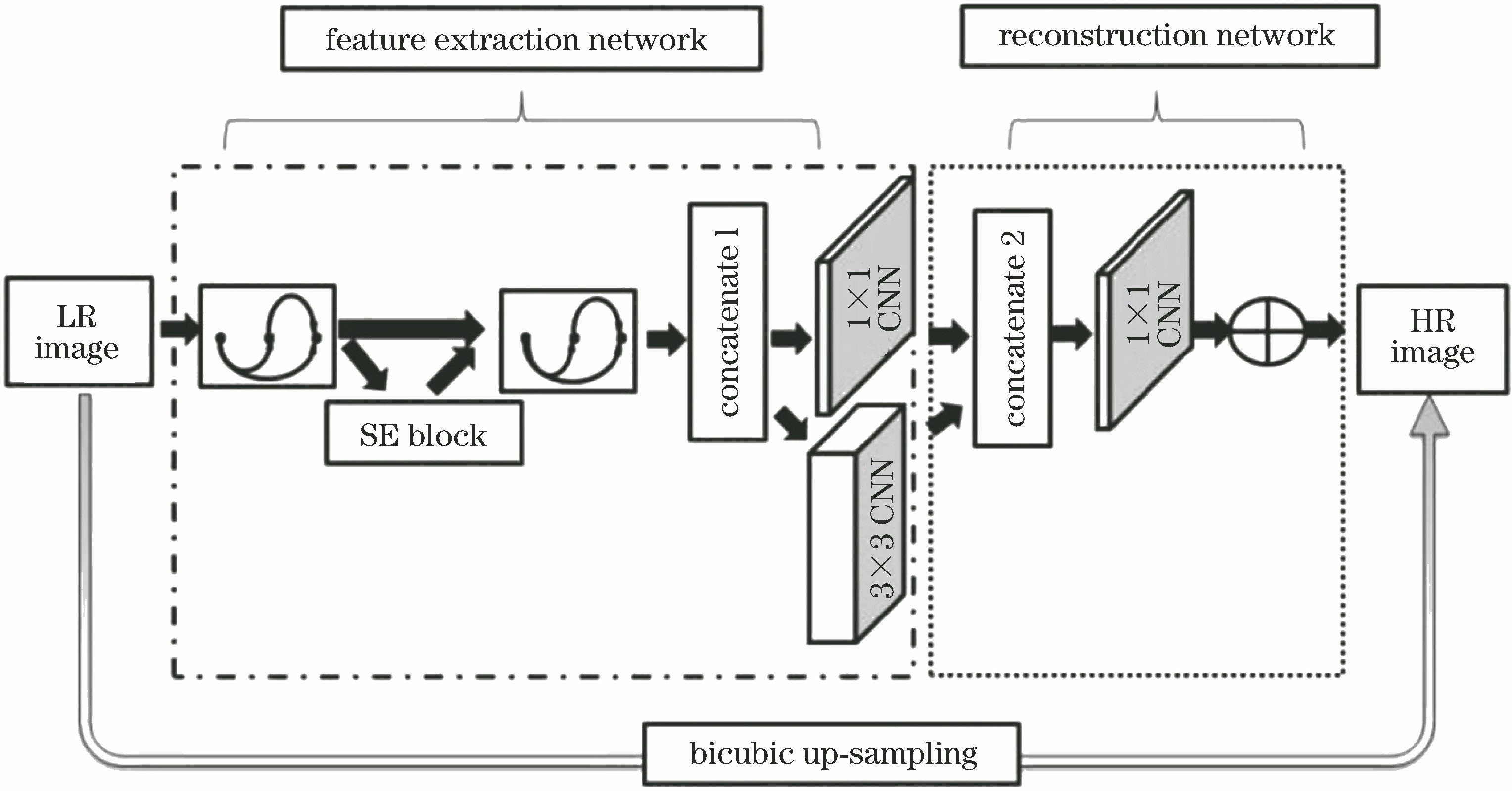
Fig. 2. Structure of DSSR

Fig. 3. Structure of dense block

Fig. 4. Structure of squeeze module

Fig. 5. Example of image data augmentation. (a) Original image; (b) horizontal flip image; (c) rotate 180° image; (d) vertical flip image

Fig. 6. Image decomposition map. (a) Decomposed image of Y channel; (b) decomposed image of Cb channel; (c) decomposed image of Cr channel

Fig. 7. Nonlinear output of different images. (a) Nonlinear output of nature image; (b) nonlinear output of text image; (c) nonlinear output of building image; (d) nonlinear output of person

Fig. 8. Nonlinear feature maps of feature extraction and image reconstruction. (a) Nonlinear mapping part feature map of the first convolution layer; (b) nonlinear mapping part feature map of the first concatenate layer

Fig. 9. Super-resolution results of “img_020” (bsd100) with scale factor ×2. (a) Original image; (b) result from Bicubic[28]; (c) result from A+[37]; (d) result from SRCNN[12]; (e) result from WSD-SR[38]; (f) result from VDSR[15]; (g) result from DRCN[39]; (h) result from LapSRN[40]; (i) result from DCSCN[19]; (j) DSSR

Fig. 10. Super-resolution results of “img_003” (Set5) with scale factor ×3. (a) Original image; (b) result from Bicubic; (c) result from A+; (d) result from SRCNN; (e) result from WSD-SR; (f) result from VDSR; (g) result from DRCN; (h) result from LapSRN; (i) result from DCSCN; (j) DSSR

Fig. 11. Super-resolution results of “img_012” (Set14) with scale factor×4. (a) Original image; (b) result from Bicubic; (c) result from A+; (d) result from SRCNN; (e) result from WSD-SR; (f) result from VDSR; (g) result from DRCN; (h) result from LapSRN; (i) result from DCSCN; (j) DSSR

Table 1. Some parameters fine-tuned (number of dense blocks, number of filters) when the scale factor is 3. Bold fonts indicate the best performance

Table 2. Technical implementation and parameter details of each super-resolution algorithm

Table 3. Average PSNR and time of different scale factors on the four benchmark datasets Set5, Set14, B100 and Urban100 (Bold fonts indicate the best performance)