Blind spectral deconvolution algorithm for Raman spectrum with Poisson noise

Hai Liu; Zhaoli Zhang; Jianwen Sun; and Sanya Liu

doi:10.1364/PRJ.2.000168

Abstract

A blind deconvolution algorithm with modified Tikhonov regularization is introduced. To improve the spectral resolution, spectral structure information is incorporated into regularization by using the adaptive term to distinguish the spectral structure from other regions. The proposed algorithm can effectively suppress Poisson noise as well as preserve the spectral structure and detailed information. Moreover, it becomes more robust with the change of the regularization parameter. Comparative results on simulated and real degraded Raman spectra are reported. The recovered Raman spectra can easily extract the spectral features and interpret the unknown chemical mixture.

Keywords

high-resolution Raman Inverse problems Spectroscopy

Raman spectra often suffer from common problems of bands overlapping and Poisson noise ^[1,2]. Raman spectra measured by a spectrophotometer can be mathematically modeled as $g (v) = Poisson (s (v) \otimes h (v)),$ (1)where $g (v)$ and $s (v)$ are the measured Raman spectrum and actual spectrum, and $h (v)$ stands for the instrument function, which mainly collects the instrumental broadening. $Poisson (\cdot)$ denotes the Poisson noise. The goal of blind spectral deconvolution is to seek the best estimates of $s (v)$ and $h (v)$ based on measured spectrum $g (v)$ and prior information about the actual spectrum scene. Over the years, many deconvolution methods have been developed, such as high-order statistic ^[3], Fourier self-deconvolution (FSD) ^[4], the Wiener filtering method ^[5], maximum entropy deconvolution ^[6], and the semi-blind deconvolution method ^[7,8]. In ^[9], Katrasnik et al. extended the Richardson–Lucy (RL) method to the spectroscopy field. Nevertheless, owing to the ill-posed nature of inverse problems, this algorithm often lacks stability and uniqueness. The amount of noise will increase with the iteration process. And the algorithm must be stopped before the noise rises above a certain level. Tikhonov regularization (TR) was initially introduced as a regularizer for spectral processing in ^[10,11]. Since then it has been used extensively and with great success for inverse problems because of its ability to suppress noise.

The maximum a posteriori (MAP) technique is a commonly used approach to estimate the actual spectrum $s (v)$ given the measured spectrum $g (v)$ . This technique maximizes the conditional probability of an actual spectrum given a certain measured spectrum. Based on Bayes’s rule, MAP can be converted to one likelihood probability multiplied by two priori probabilities. In this paper, the MAP framework is employed to construct the spectral deconvolution model. Considering the cases in which the data are contaminated by Poisson noise, the intensity of each pixel $g (v)$ in the measured spectrum is a random variable that obeys an independent Poisson distribution. Hence the likelihood probability can be written as $p (g | s, h) = \prod_{v}^{L} \frac{{(s (v) \otimes h (v))}^{g (v)}}{g (v)!} \exp {(- s (v) \otimes h (v))},$ (2)where $L$ denotes the spectral length.

To estimate $s$ and $h$ , iterative deconvolution algorithms can be used. One option is to use the RL method ^[9], which minimizes the following functional to maximize Eq. (2): $E_{1} (s) = \sum_{v} (- g (v) \log [s (v) \otimes h (v)] + s (v) \otimes h (v)) .$ (3)

Sign up for Photonics Research TOC. Get the latest issue of Photonics Research delivered right to you！Sign up now

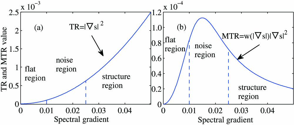
The RL algorithm does not converge to the solution because the noise is amplified after a small number of iterations. In order to get better convergence, the RL method with Tikhonov regularization ^[11] (TR-RL) was proposed, and the cost functional to be minimized is then $E_{2} (s) = \sum_{v} (- g (v) \log [s (v) \otimes h (v)] + s (v) \otimes h (v)) + α {| \nabla s |}^{2},$ (4)where $\nabla s = (s_{i} - s_{i + 1}) / 2$ . Symbol $α$ is the regularization parameter, which plays a very important role, controlling the constraint strength. If $α$ is too small, the noise will not be well suppressed; conversely, if it is too large, the spectral structure will be removed. This means that the regularization parameter $α$ needs to be adaptively adjusted according to spectral structure information. For better structure information preservation, in the TR term, we added a nonnegative monotonically decreasing function $w (| \nabla s |)$ to control the regularization about the spectrum ^[12]: $w (| \nabla s |) = \frac{1}{1 + {(\nabla s / k)}^{2}},$ (5)where $k$ is a constant between 0.01 and 1. Combining the adaptive term $w (| \nabla s |)$ into the TR model, the modified Tikhonov regularization (MTR) model with spectral structure information is defined: $MTR = w (| \nabla s |) {| \nabla s |}^{2},$ (6)which can distinguish three types spectral regions (flat, noise, and structure regions), but TR cannot distinguish those regions. The difference is shown in Fig. 1. Substituting the TR term in Eq. (4) with MTR in Eq. (6), we introduce the total functional: $E (s, h) = \sum_{v}^{L} [- g (v) \log (s (v) \otimes h (v)) + s (v) \otimes h (v)] + α w (| \nabla s |) {| \nabla s |}^{2} .$ (7)

Illustration of TR and MTR constraints on three types: flat region, noise region, and structure region. (a) Tikhonov regularization. (b) Modified Tikhonov regularization can distinguish different regions.

Figure 1.Illustration of TR and MTR constraints on three types: flat region, noise region, and structure region. (a) Tikhonov regularization. (b) Modified Tikhonov regularization can distinguish different regions.

Minimizing Eq. (7) by the expectation maximization (EM) algorithm, the numerical iterative algorithm is then obtained, ${\hat{s}}_{t}^{(k + 1)} = {\hat{s}}^{(k)} {{\hat{h}}^{(k)} (- v) \otimes [\frac{g}{{\hat{s}}^{(k)} \otimes {\hat{h}}^{(k)}}]}, {\hat{s}}^{(k + 1)} = \frac{{\hat{s}}_{t}^{(k + 1)}}{\sum_{v} {\hat{s}}_{t}^{(k + 1)}},$ (8) ${\hat{h}}_{t}^{(k + 1)} = {\hat{h}}^{(k)} {{\hat{s}}^{(k + 1)} (- v) \otimes [\frac{g}{{\hat{s}}^{(k + 1)} \otimes {\hat{h}}^{(k)}}]} \times \frac{1}{{1 - α w (| \nabla \hat{s} |) (\nabla^{2} \hat{s})}},$ (9)where the superscript indexes the number of the iteration. The term $w (| \nabla \hat{s} |)$ is calculated by the previous iteration result ${\hat{s}}^{(k)}$ .

Summarizing, two good advantages of MTR-RL can be drawn: (i) for the flat region because $w (| \nabla \hat{s} |)$ is close to 1, which means a large TR strength is enforced to these points, and then the noise will be suppressed; (ii) for structure regions because $w (| \nabla \hat{s} |)$ is small and almost close to 0 and weakens the TR strength, so the spectral detail and structure will be preserved. In other words, MTR-RL has the ability to adaptively adjust the regularization strength according to the spectral structure information.

To quantitatively evaluate the deconvoluted spectra, three metrics, the normalized mean square error (NMSE) ${‖ s - \hat{s} ‖}^{2} / {‖ s ‖}^{2}$ , the full width at half-maximum ratio (FWHMR) $\frac{1}{N} \sum_{i}^{N} {FWHM}_{g}^{(i)} / {FWHM}_{s}^{(i)}$ ^[9], and the noise suppression ratio (NSR) $\sum | \nabla g | / | \nabla \hat{s} |$ , are employed. ${FWHM}_{g}^{(i)}$ and ${FWHM}_{\hat{s}}^{(i)}$ are the widths of the bands in the measured spectrum $g$ and deconvoluted spectrum $\hat{s}$ , respectively. NSR was defined as the ratio of the total variation of the measured spectrum $g$ to the total variation of the deconvoluted spectrum $\hat{s}$ , which is the noise attenuation measure. Among these three metrics, the NMSE requires the existence of a reference spectrum $s$ . Therefore, it can only be used in simulated experiments. FWHMR and NSR, which are nonreference measures of spectra, can also be used in experiments performed on real Raman spectra. It has been verified that the two metrics can reflect the width reduction and noise suppression ^[9]. The larger the values of FWHMR and NSR, the higher the spectral quality.

To demonstrate the effectiveness of the proposed method, we execute simulations with three test spectra under the Poisson noise process. The spectra come from the demo spectral library of Bruker Optics Incorporation. They were degraded by a Gaussian function with standard variance 12 [shown in Fig. 2(b)]. The degraded spectrum becomes much smoother and less resolved, in which the bands become wider and lower. For instance, it is difficult to distinguish the peak at $1215 {cm}^{- 1}$ from that at $1163 {cm}^{- 1}$ . Then the overlap spectrum was contaminated by Poisson noise [illustrated in Fig. 2(c)]. Three type regions can be defined according to the spectral gradient value, which is shown in Fig. 1. For comparison, the FSD, RL, and TR-RL methods were adopted.

Figure 2.Simulation experiment. (a) Raman spectrum of methyl formate ( $C_{2} H_{4} O_{2}$ ) from 400 to $1500 {cm}^{- 1}$ . (b) Overlap spectrum. (c) Contaminated by Poisson noise. (d) RL. (e) TR-RL. (f) MTR-RL.

Figures 2(d)–2(f) show a simulation example of restoration by RL, TR-RL, and MTR-RL. We chose $α = 0.05$ and 200 iterations. Comparing Fig. 2(d) with Fig. 2(f), it can be found that MTR-RL obviously reduces the artifacts as well as better preserves the spectral structure. The effects of the regularization parameter were also investigated. For the TR-RL and MTR-RL methods, the NMSE of the deconvoluted spectrum versus varying regularization parameter $α$ on the simulated degraded spectrum of Fig. 2(c) is plotted in Fig. 3. The MTR-RL method appears more robust with the change of the regularization parameter at a wide range from $10^{- 1.75}$ to $10^{- 1}$ at intervals of 0.005. However, the change of regularization parameter $α$ has a great impact on the performance of TR-RL. In particular, the NMSE value increases dramatically when the regularization parameter becomes large.

Figure 3.NMSE versus regularization parameter of TR-RL and MTR-RL for the Raman spectrum of methyl formate ( $C_{2} H_{4} O_{2}$ ).

Moreover, the NMSE of degraded spectra and the best deconvolution spectra by the three methods are compared in Table 1. The best deconvolution spectrum is selected to be the one with the lowest NMSE when the regularization parameter changes. It can be seen that the MTR-RL method has achieved the smallest NMSE among the three methods. The NMSE versus the number of iterations by the three methods on the Raman spectrum [methyl formate ( $C_{2} H_{4} O_{2}$ )] is shown in Fig. 4, where the convergence is also highlighted.

Figure 4.NMSE versus the iteration number of the three methods for the Raman spectrum [methyl formate ( $C_{2} H_{4} O_{2}$ )].

		Spectral Deconvolution by
Spectra	Degraded Spectrum	FSD [4]	RL [9]	TR-RL	MTR-RL
C2H4O2	0.0451	0.0272	0.0231	0.0240	0.0219
C9H10O2	0.0223	0.0195	0.0136	0.0105	0.0092
C4H4S	0.0480	0.0315	0.0231	0.0198	0.0184

Table 1. NMSE of Measured Spectrum and the Best Deconvolution Spectrum (with the Lowest NMSE by Different Algorithms)

View all Tables

Finally, the proposed algorithm was applied to real Raman spectra. Owing to photon-limited detection, Raman spectra are always corrupted by Poisson noise. We tested eight Raman spectra, which are downloaded from ^[13,14]. We use $α = 0.05$ , starting with a 69 nm Gaussian function with a standard deviation of 2 for the initial instrument function. In order to save space, only two of them are illustrated. Figure 5(a) shows the 600 length spectrum of Cr:LisAF crystal from 300 to 900 nm. The two peaks at 631 and 661 nm overlap each other, and only two pinnacles can be distinguished. Figures 5(b) and 5(c) are the deconvoluted results by TR-RL and MTR-RL. The two peaks at 631 and 661 nm are split into four peaks at 580, 604, 631, and 663 nm, respectively. However, the TR-RL result only has three peaks. The instrument function is plotted in Fig. 5(d), whose width is about 69 nm.

Figure 5.Real Raman spectrum experiment. (a) Cr:LisAF crystal [13] from 300 to 900 nm, deconvolution by (b) TR-RL and (c) MTR-RL. (d) Estimated instrument function.

Figure 6(a) shows the 690 length Raman spectrum of (D+)-glucopyranose ^[14] from 10 to $700 {cm}^{- 1}$ . Figure 6(b) shows the deconvolution data. Here we choose $α = 0.05$ . The peak at $406 {cm}^{- 1}$ is split into two peaks at 395 and $406 {cm}^{- 1}$ , respectively, and the peak at $542 {cm}^{- 1}$ is separated into two peaks at 542 and $557 {cm}^{- 1}$ , respectively. The spectral resolution has been improved considerably, and the distortion of the relative intensity can be revised to some degree. The same spectrum has been deconvoluted by ^[15], but the deconvoluted result seems rather noisy. Table 2 shows the FWHMR and NSR values of all the eight Raman spectra. It is seen that all the blind deconvolution methods raise the FWHMR and NSR, but the proposed method obtains the highest values.

Figure 6.Real Raman deconvolution experiment. (a) Raman spectrum of (D+)-glucopyranose [14] from 10 to $700 {cm}^{- 1}$ . (b) MTR-RL result.

Spectrum	FSD[4]	RL[9]	TR-RL	MTR-RL
Raman 1	1.47	1.50	3.61	3.98
Raman 1	(1.10)	(1.32)	(2.20)	(2.35)
Raman 2	1.67	2.28	4.50	4.71
Raman 2	(1.18)	(1.91)	(2.18)	(2.46)
Raman 3	1.25	1.78	3.61	3.81
Raman 3	(1.68)	(1.71)	(2.22)	(2.31)
Raman 4	1.87	2.21	2.90	3.04
Raman 4	(1.41)	(1.75)	(2.31)	(2.40)
Raman 5	1.45	2.16	2.85	3.29
Raman 5	(1.02)	(1.01)	(1.80)	(1.96)
Raman 6	1.88	2.43	3.01	3.21
Raman 6	(1.10)	(1.22)	(1.56)	(1.76)
Raman 7	1.71	1.98	2.50	2.61
Raman 7	(1.24)	(1.31)	(1.68)	(2.01)
Raman 8	1.42	1.68	2.31	2.58
Raman 8	(1.89)	(2.11)	(2.48)	(2.86)

Table 2. FWHMR and NSR (in Brackets) Values of Different Deconvolution Methods on the Real Raman Spectraa

View all Tables

This paper has presented a new spectral blind deconvolution method for Raman spectrum with Poisson noise. The proposed method can automatically balance the regularized strength between different spectral structures. Comparative results on simulated and real spectra show that MTR-RL can effectively reduce the Poisson noise and preserve the spectral structure information. Moreover, it becomes more robust with the regularization parameter, which makes the method more preferable in practical applications. The recovered Raman spectra can easily extract the spectral features and interpret the unknown chemical mixture. Although the application considered here is Raman spectroscopy, the method is more generally applicable to fluorescence data, and so on.

Nevertheless, there may still be room for improvement in our proposed method. In fact, the instrumental broadening usually varies with wavenumber in dispersive Raman spectrometers, because of the monochromator. Thus, the instrument function $h (v)$ is not necessarily unique. We will examine this in our future work.

References

[1] J. J. Weber, D. D. Yavuz. Broadband spectrum generation using continuous-wave Raman scattering. Opt. Lett., 38, 2449-2451(2013).

[2] K. Y. Song, H. J. Yoon. Observation of narrowband intrinsic spectra of Brillouin dynamic gratings. Opt. Lett., 35, 2958-2960(2010).

[3] J. Yuan, Z. Hu, J. Sun. High-order cumulant-based blind deconvolution of Raman spectra. Appl. Opt., 44, 7595-7601(2005).

[4] J. K. Kauppinen, D. J. Moffatt, H. H. Mantsch, D. G. Cameron. Fourier self-deconvolution: a method for resolving intrinsically overlapped bands. Appl. Spectrosc., 35, 271-276(1981).

[5] C. W. Helstrom. Image restoration by the method of least squares. J. Opt. Soc. Am., 57, 297-303(1967).

[6] V. A. Lórenz-Fonfría, E. Padrós. Maximum entropy deconvolution of infrared spectra: use of a novel entropy expression without sign restriction. Appl. Spectrosc., 59, 474-486(2005).

[7] L. Yan, H. Liu, S. Zhong, H. Fang. Semi-blind spectral deconvolution with adaptive Tikhonov regularization. Appl. Spectrosc., 66, 1334-1346(2012).

[8] H. Liu, T. Zhang, L. Yan, H. Fang, Y. Chang. A MAP-based algorithm for spectroscopic semi-blind deconvolution. Analyst, 137, 3862-3873(2012).

[9] J. Katrasnik, F. Pernu, B. T. Likar. Deconvolution in acousto-optical tunable filter spectrometry. Appl. Spectrosc., 64, 1265-1273(2010).

[10] F. Stout, J. H. Kalivas, K. Héberger. Wavelength selection for multivariate calibration using Tikhonov regularization. Appl. Spectrosc., 61, 85-95(2007).

[11] D. K. Buslov, N. A. Nikonenko. Regularized method of spectral curve deconvolution. Appl. Spectrosc., 51, 666-672(1997).

[12] L. Z. Deng, L. Cao, H. Zhu. Spectral semi-blind deconvolution with hybrid regularization. Infrared Phys. Technol., 64, 91-96(2014).

[13] . Absorption spectral data of Cr:LiSAF crystal.

[14] S. B. Engelson. Raman spectral of (D+)-glucopyranose.

[15] J. Yuan, Z. Hu, G. Wang, Z. Xu. Constrained high-order statistical blind deconvolution of spectral data. Chin. Opt. Lett., 3, 552-555(2005).