• Journal of Geographical Sciences
  • Vol. 30, Issue 10, 1649 (2020)
Yongqiang ZHANG*
Author Affiliations
  • Key Laboratory of Water Cycle and Related Land Surface Processes, Institute of Geographic Sciences and Natural Resources Research, CAS, Beijing 100101, China
  • show less
    DOI: 10.1007/s11442-020-1805-9 Cite this Article
    Yongqiang ZHANG. Using LiDAR-DEM based rapid flood inundation modelling framework to map floodplain inundation extent and depth[J]. Journal of Geographical Sciences, 2020, 30(10): 1649 Copy Citation Text show less

    Abstract

    Mapping floods is important for policy makers to make timely decisions in regards to emergency responses and future planning. It is therefore crucial to develop a rapid inundation modelling framework to map flood inundation. This study develops an airborne scanning laser altimetry (LiDAR) digital elevation model (DEM) based Rapid flood Inundation Modelling framework (LiDAR-RIM) for assessment of inundation extent, depth, volume and duration for flood events. The modelling framework has been applied to the mid-Murrumbidgee region in the southeast Murray-Darling Basin, Australia for two flood events occurred in December 2010 and March 2012. The inundation extents estimated using this methodology compared well to those obtained from two Landsat ETM+ images, demonstrating suitability and applicability of this method. For testing possibility of larger area application, the framework also uses 30-m resolution shuttle radar topography mission (SRTM)-DEM to replace LiDAR-DEM for the same modelling. The inundation extents obtained by using the SRTM-DEM are smaller than those obtained using the LiDAR-DEM, especially for large flood events. A possible reason is that the river cross sections obtained from the SRTM-DEM are not accurate enough for inundation modelling. The LiDAR-RIM has an advantage for process modelling and scenario modelling under future climatic conditions.

    1 Introduction

    Mapping floodplain inundation extent and depth is critical for the management of river systems, environmental assessment and disaster management (Sanyal and Lu, 2004; Penton and Overton, 2009; Huang et al., 2014; Saksena and Merwade, 2015). In many large basins across the world, such as the Murray-Darling Basin (MDB) in southeast Australia, there are a large number of wetlands along the rivers. The environmental benefits of water flowing into wetlands and over floodplains depends on the understanding of the extent, depth, duration and frequency of the inundation (Penton and Overton, 2009). On the other hand, floods are one of most devastating natural hazards in many parts of the world, damaging crops and infrastructures and threatening human lives. To formulate a reliable flood management strategy, the first step is to identify the possible inundation extent and depth for flood events (Sanyal and Lu, 2004).

    Two widely used approaches for inundation mapping are hydrodynamic modelling based on water equilibrium equations and flood mapping using remote sensing images. Hydrodynamic modelling uses water equilibrium equations to simulate water movement along river channels and overbank flow (Wu et al., 2017). The representative hydrodynamic models include MIKE (Thompson et al., 2004), HEC-RAS (Horritt and Bates, 2002; Pappenberger et al., 2005) and LISFLOOD-FP (Bates and De Roo, 2000). These models require accurate high-resolution DEM cross-sections of river channels and cross-sections of floodplains. These models simulate water movement in river channels and floodplains and estimate their inundation extent, duration, depth and frequency of wetting by using water equilibrium equations, such as St. Venant’s equations. They can also be used for analyzing impacts of modification of control structures such as levee banks. However, they are computationally expensive and need detailed parameter information (for each grid cell) for model calibration. In other words, it is hard to apply if detailed parameter information is not available. Using remote sensing images to map inundation extents has received considerable attention over large areas since they are computationally cheap and relatively accurate (Bates et al., 1997; Smith, 1997; Shaikh et al., 2001). Satellite and airborne platforms can be used for mapping surface water bodies and flood inundation extents (Tseng et al., 2016; Jiang et al., 2017; Zheng et al., 2017; Busker et al., 2019; Johnson et al., 2019; Li et al., 2019). The flood maps can act as validation datasets for hydraulic flood inundation models. There are two kinds of remote sensing images: (1) passive remote sensing images obtained from Landsat Thematic Mapper (TM) and Enhanced TM (ETM+), ERS1 and ERS2, and RADARSAT; and (2) active microwave radar images, such as Synthetic Aperture Radar (SAR) imagery. Bates et al. (1997) and Smith (1997) reviewed the active and passive remote sensing studies of flood inundation. Shaikh et al. (2001) classified wetlands of the Lower Darling River in southeastern Australia by using broad commence-to-flow discharges and the inundation effects at different discharge magnitudes. To date, remote sensing of floodplain inundation from satellite platforms have not yet offered a solution to the dynamic flood inundation processes due to coarse temporal resolution (e.g. 35 days for ERS1 and ERS2 satellites, 14 days for Landsat, 7 to 10 days for RADARSAT). Furthermore, successful application of passive remote sensing data depends on cloudless conditions and open canopy cover (Wang et al., 2002). The passive remote sensing data, such as Landsat and ERS1 and ERS2 satellites cannot penetrate clouds and dense vegetation canopy (Bate et al., 1997; Smith, 1997). Another issue for remote sensing inundation observations is that it is hard to distinguish existing water bodies in wetlands/floodplains from the flood inundation extension. Nevertheless, inundation maps extracted from remote sensing images indeed provide very useful validation datasets for the flood inundation models that can simulate a variety of historical and likely future conditions.

    Use of high-resolution airborne scanning laser altimetry (LiDAR) digital elevation model (DEM) data for flood inundation modelling has also received lots of attention for floodplain/wetland inundation mapping and the river network study since they are of high resolution (1 m or 2 m) and can capture the river network reasonably accurately (Cook and Merwade, 2009; Vaze et al., 2010; Negishi et al., 2012; Smith et al., 2012; Tsubaki and Kawahara, 2013; Teng et al., 2015; Chen et al., 2017). Sanders (2007) used the LiDAR-DEM and other several DEM products (airborne interferometric synthetic aperture radar (IfSAR), national elevation data (NDE), and shuttle radar topography mission (SRTM)) to parameterize a 2D hydrodynamic flood model, respectively. He found that the inundation extent simulated using the LiDAR-DEM is much better than that simulated using other DEM products, when both are compared with the published flood maps. Zwenzner and Voigt (2009) presented a methodology to improve the matching of flood masks with the high resolution (1 m and 2 m) LiDAR-DEM. Penton and Overton (2009) used the LiDAR-DEM together with a simple GIS-based inundation model for inundation mapping along the lower Murray River and the simulated result compared well with the inundation maps generated from Landsat TM/ETM images. Chen et al. (2017) further demonstrated that LiDAR technology performed well for mapping the 2008 Iowa flood in the United States, and is a great benchmark source to evaluate accuracy from other inundation modelling.

    Location of research area (a); spatial pattern of 2-m resolution LiDAR-DEM and locations of the three gauges (b)

    Figure 1.Location of research area (a); spatial pattern of 2-m resolution LiDAR-DEM and locations of the three gauges (b)

    One limitation of the LiDAR-DEM is that it is only currently available for the small floodplain/wetland regions. For large area application, the inundation modelling framework needs the help of other relative coarse resolution DEM dataset, such as 1-sec SRTM-DEM dataset which is freely available globally (http://srtm.usgs.gov/). Sanders (2007) showed that using 1 sec and 3 sec SRTM-DEM for estimating inundation extent got noticeably different results. The SRTM-DEM failed to capture a channel 300 m wide in the Buffalo Bayou. In addition to errors from the radar speckle, 1-sec and 3-sec STRM-DEMs may have data gaps caused by radar shadow, which makes them unsuitable for flood modelling. The SRTM-DEM data, however, shows remarkable value for the Santa Clara River which is only 200 m wide. Therefore, it is necessary to further investigate the usability of the SRTM-DEM data for inundation modelling.

    This study develops a LiDAR-DEM based Rapid Inundation Modelling framework, named as LiDAR-RIM. It overcomes the issues associated with hydrodynamic modelling (e.g., slow computation) and remote sensing mapping (e.g., clouds, dense canopies and flood water mixed with water bodies). To take advantage of the high resolution LiDAR-DEM data, the LiDAR-RIM used the LiDAR-DEM together with gauging site information, loss/gain functions, flow data, climate and floodplain soil property to quickly model floodplain inundation extents, depths, volumes (for any given river stage and to simulate the relationship between river stage) and inundation area. The modelling framework was tested for two flood events and at two mid Murrumbidgee river reaches in the southeastern MDB (Figure 1). The modelled inundation extents were compared to observations from the Landsat ETM+ images. In addition, the LiDAR-FIM used 1-sec SRTM-DEM data to replace LiDAR-DEM for the same modelling, and the corresponding results were evaluated against the observations.

    2 Modelling framework and data

    2.1 LiDAR-RIM

    The LiDAR-RIM was developed for quick assessment of flood inundation extent, depth, volume and duration for any high flow event based on LiDAR-DEM data and simple hydraulic principles of mass balance (Figure 2). There are seven major steps involved in the modelling framework as follows:

    1) Multiple LiDAR-DEM files are mosaiced along the mid Murrumbidgee River reaches.

    2) River networks are digitized using the mosaiked LiDAR-DEM dataset.

    Flowchart showing how the LiDAR - RIM framework works

    Figure 2.Flowchart showing how the LiDAR - RIM framework works

    3) Using the LiDAR-DEM obtains river cross section for a given gauging site (Figure 3), estimates the inundations depth between LiDAR-DEM water surface and water surface for a given flood event, and then generates the maps of flood water surface and inundation depth (flood water surface minus LiDAR- DEM).

    An example for estimating inundation depth from the 2 m LiDAR-DEM water surface to flood water surface at the gauge site 410005

    Figure 3.An example for estimating inundation depth from the 2 m LiDAR-DEM water surface to flood water surface at the gauge site 410005

    4) The initial constrained inundation extent and inundation depth are calculated using mass balance (Equation (1)) and the corresponding inundation volume estimated from the difference between the cumulative flow at the two gauges minus the losses between the two gauges estimated from loss/gain functions in the simplified MDB daily river model (Hughes et al., 2012; Hughes et al., 2014). The river bursts from the lowest cross section point, water spreads over the floodplain, and stops when the corresponding inundation volume is reached (Figure 4). The extent at the stop time is regarded as the initial inundation extent and corresponding inundation depths for the inundated grid cells are calculated (flood water surface minus LiDAR-DEM).

    5) Flood extent and flood depth at each grid cell change from the initial inundation (see step 4) by adding losses due to infiltration (estimated using soil properties) and open water evaporation (estimated from daily climate data after the flood events). For each grid cell, the flood depth gradually reduces, and it reduces to zero once the total depth of infiltration and water evaporation is as same as or larger than the initial flood depth.

    6) Inundation extent obtained by LiDAR-RIM is compared to that obtained by Landsat TM/ETM+ images from which the normalised difference water index (NDWI) is mapped (McFeeters, 1996). It is then used to identify open water bodies and corresponding inundation areas.

    7) Inundation extents and inundation volumes are simulated at different flood level scenarios.

    Step 4 is key, and the mass balance is expressed as:

    ${{Q}_{d}}=({{Q}_{u}}+{{Q}_{g}}-{{Q}_{l}})+{{Q}_{ungauged}}-loss+\varepsilon ,$

    where Qd is the estimated streamflow at the down streamflow gauge, Qu is the concurrent streamflow at the upstream gauge, Qg is any explicit gains (e.g. channel precipitation), Ql is any explicit losses (e.g. irrigation diversions and channel evaporation), Qungauged is inflow from the ungauged contribution area, loss means unaccounted gains or losses and ɛ is error. This equation is calibrated at each reach using an automatic calibration scheme developed by Hughes et al. (2014).

    A schematic figure showing flood flow directions over the floodplain

    Figure 4.A schematic figure showing flood flow directions over the floodplain

    The LiDAR-FIM was developed in MATLAB by using high performance computation clusters to handle a large DEM matrix with a size up to about 20000×20000 grid cells (about 1600 km2 for 2-m resolution LiDAR-DEM). It took about 3-5 hours for the LiDAR-RIM to map the constrained inundation extent and depth for 20000×20000 grid cells.

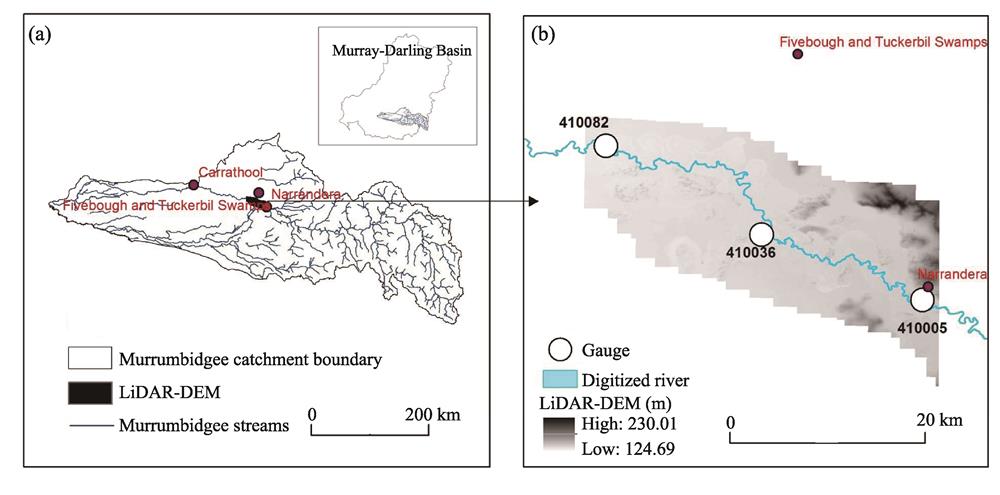
    2.2 Study area and data

    The study area is located in the lower Murrumbidgee floodplain along the Murrumbidgee River (Figure 1a), a major tributary of the Murray River within the MDB. This area is environmentally important since it is covered by a lot of wetlands in the mid Murrumbidgee and by riparian forests along the Murrumbidgee River from near Narrandera to Carrathool (Doody et al., 2015). These wetlands are nationally and internationally important and the non-riparian Fivebough and Tuckerbil Swamps near Leeton are listed in the Ramsar wetlands list (EA, 2001). The wetlands are on the floodplain and receive water from the river systems during flood periods.

    The LiDAR-RIM was applied for inundation modelling in the study area. Two wetland reaches were selected: one from gauging site 410005 to 410036; another from gauging site 410036 to 410082 (Figure 1b). The raw LiDAR XYZ files were provided by the New South Wales (NSW) Office of Environment and Heritage. The XYZ files were first converted into Geotiff files at different spatial resolutions varying from 2 m to 40 m. The 2-m resolution DEM was taken as a benchmark to evaluate performance of the coarse resolution LiDAR-DEM.

    Some preliminary processes were conducted for the LiDAR-DEM before forcing the LiDAR-RIM. First, individual files were mosaiked (Figure 1b). Then, the mosaiked DEM was destriped using the nearest neighbouring interpolation methods because several stripes were identified after the mosaiking. After that, the LiDAR-DEM data, at different resolutions, were inputted into the LiDAR-FIM for inundation modelling.

    The 1-sec (approximately 30-m) resolution SRTM-DEM product was provided by Geoscience Australia (Gallant et al., 2011). This product included: a cleaned digital surface model (DSM), a bare-earth DEM, a smoothed DEM (DEM-S) and a hydrologically enforced DEM (DEM-H). This study used DEM-H because it is based on DEM-S that has imposed drainage lines and has been smoothed using the ANUDEM interpolation software (Hutchinson, 2009).

    Two flood events were tested in December 2010 and March 2012. The December 2010 flood in the Murrumbidgee River has a return period of ~10 years. The flood started on December 11 and continued until December 22 in this region, with the peak flow occurring on December 18. The March 2012 flood has a return period of ~100 years. The flood started on March 7 and continued until March 14 at this region, with the peak flow occurring on March 9. The Landsat ETM+ image for 2012 flood inundation mapping was taken on March 20, 2012, 6 days after the flood event. The Landsat ETM+ image for the 2010 flood inundation mapping was taken on January 5, 2011, 12 days after the flood event. Both were obtained from Earth Resources Observation and Science Center (http://glovis.usgs.gov/), U.S. Geological Survey (USGS). Both were cloud free but the ETM+ image taken on March 20, 2012 was with stripes for which no data was available. To obtain the stripe-free ETM+ image, the stripes were filled using the nearest neighbouring interpolation algorithm. The image covers the whole inundation extent and is suitable for this flood modelling.

    The real-time streamflow data and gauging information at the three gauges of 410045, 410036 and 410082 were obtained from the NSW Government WaterInfo website (http://waterinfo.nsw.gov.au/). Gauging information includes gauge latitude/longitude, zero flow gauge, maximum river stage and date, etc.

    To estimate open water evaporation and local precipitation input for inundation modelling, local climate data including daily precipitation and potential evaporation data was obtained from the Bureau of Meteorology through its free climate data online (http://www.bom.gov.au/climate/data-services/#).

    To estimate infiltration, the soil property data for the selected reaches were obtained from a subset of Australian soil property GIS databases which was produced by CSIRO (McKenzie et al., 2000). The soil property data includes saturated hydrological conductivity for the surface and sub-surface soil layers which was used for infiltration estimation.

    3 Results and discussion

    3.1 Inundation depth across gauging sites

    Table 1 summarises the maximum inundation depth for the three gauging sites. For the March 2012 flood (occurring once every 100 years), the inundation depth for the gauging sites 410005, 410036 and 410082 were 7.05 m, 6.62 m, 6.64 m, respectively; for the December 2010 flood (occurring once every 10 years), the depth for the gauging sites 410045, 410036 and 410082 were 6.09 m, 6.08 m and 6.27 m, respectively. This result indicates the inundation depths are relatively stable across the three gauging sites and along the two reaches. Therefore, for a given flood event, a universal inundation depth, averaged over the two gauges, is applied to the digitized river to generate maps of the inundated water surface, maximum inundation depth, and maximum inundation extent. The universal value for each reach and each flood event is given in Table 1.

    Gauging site or digitized reachDepth from zero gauge to LiDAR- DEM (m)Maximum river stage (m)Maximum inundation depth (m)
    December 2010 floodMarch 2012 floodDecember 2010 floodMarch 2012 flood
    Gauging site4100051.97.998.956.097.05
    4100361.37.387.926.086.62
    4100820.97.177.546.276.64
    Digitized reach410005-410036--6.086.84
    410036-410082--6.186.63

    Table 1.

    Inundation depth for the three gauging sites and for the two flood events. Maximum inundation depth is the difference between maximum river stage and the depth from zero gauge to the LiDAR-DEM water surface.

    3.2 Flooding mapping using LiDAR-FIM

    Figure 5 shows the maximum possible inundation extent and depth for the two flood events in March 2012 (Figure 5a) and December 2010 (Figure 5b), which were obtained under unlimited water supply from the river. The maximum inundation area for this region was about 359.8 km2 for the March 2012 flood and 347.5 km2 for the December 2010 flood. Spatial patterns of the inundation depth show that it is deeper along the river and becomes gradually shallower from the river to the outside floodplain.

    Unconstrained inundation depth mapping for March 2012 flood (a) and December 2010 flood (b)

    Figure 5.Unconstrained inundation depth mapping for March 2012 flood (a) and December 2010 flood (b)

    The results shown in Figure 5 are obtained without considering mass balance, infiltration and open water evaporation across the floodplain. Figures 6b and 6e show the inundation extent considering mass balance for the March 2012 flood (Figure 6b) and the December 2010 flood (Figure 6e). The inundation extents for the 2012 and 2010 flood events are 128.2 km2 and 38.5 km2 respectively (Table 2), which are only about 1/3 and 1/10 of the maximum extent shown in Figures 5a and 5b, respectively. Figures 6c and 6f show the inundation extent considering mass balance, infiltration and open water evaporation across the inundation area for the 2012 and 2010 floods, respectively. The estimated infiltration to reach the saturated soil water condition is 80 mm/d for this region (McKenzie et al., 2000) and the estimated open water evaporation loss is about 7.0 mm/d for the December 2010 flood and about 5.0 mm/d for the March 2012 flood. The local rainfall gain is about 8.4 mm during the 2010 flood period and about 23 mm during 2012 flood period. Therefore, the total loss of the 2010 flood from 11/12/2010 (flood starting date) to 04/1/2011 (one day before the Landsat image ETM+ was taken) is about 2,167 mm; the total loss for the 2012 flood from 8/3/2012 (flood starting date) to 19/3/2012 (flood end date 14/3/2012) is about 1,000 mm. The inundation extent shown in Figure 6c is about 112.1 km2 (for March 2012 flood) which is slightly smaller than that obtained only considering mass balance (Figure 6b), and the inundation extent in Figure 6f is 20.8 km2 (for the December 2010 flood), which is about half of the flood inundation extent obtained only with mass balance (Figure 6e). The inundation extent for the 2010 flood (Figures 6e and 6f) dropped more noticeably because the Landsat ETM+ image was taken 25 days after the flood started, compared to the image taken 13 days after the start of the 2012 flood.

    Water bodies (black) extent obtained using Landsat ETM+ images taken on March 20, 2012 (a) and January 5, 2011 (b), respectively (red polygons are the boundaries of actual inundation extent (see Figures 6c and 6f); inundation extents controlled by flood mass balance (b and d); inundation extents obtained by considering flood mass balance control together with infiltration and open water evaporation (c and f). (a)-(c) are for the March 2012 flood; (d) and (f) are for the December 2010 flood.

    Figure 6.Water bodies (black) extent obtained using Landsat ETM+ images taken on March 20, 2012 (a) and January 5, 2011 (b), respectively (red polygons are the boundaries of actual inundation extent (see Figures 6c and 6f); inundation extents controlled by flood mass balance (b and d); inundation extents obtained by considering flood mass balance control together with infiltration and open water evaporation (c and f). (a)-(c) are for the March 2012 flood; (d) and (f) are for the December 2010 flood.

    Figures 7a and 6c describe the relationships between the river stage (H) and the inundation volume (V) for the March 2012 flood and for the reaches 410005-410036 and 410036-410082, respectively. The inundation volume was obtained considering mass balance as described in step 4 in section 2.1. For the reach 410005-410036, inundation did not occur when the river stage was below 7.5 m, and inundation depth increased gradually from the river stage 7.6 m to 8.4 m, but increased sharply from the river stage 8.4 m to 8.9 m. The inundation volume for the stage below 8.4 m was about 1/3 to 1/10 of that for the stage above the 8.4 m. For the reach 410036-410082, the inundation volume was very small when the river stage was below 6.5 m. It increased gradually from the river stage of 6.5 m to 7.3 m, but increased sharply from the river stage of 7.3 m to 7.9 m. The stage-inundation relationship results shown here indicate that the inundation extent is extremely sensitive to certain stage heights, and most of the water spreads on the floodplain when the river stage is above a certain threshold (Figure 3).

    Relationships between the river stage and inundation volume (a and c); relationships between river stage and inundation area obtained using different resolutions from 2 m to 40 m (b and d). The upper panels (a), (b) and (c) are for the March 2012 flood; the lower panels (b), (c) and (d) are for the December 2010 flood.

    Figure 7.Relationships between the river stage and inundation volume (a and c); relationships between river stage and inundation area obtained using different resolutions from 2 m to 40 m (b and d). The upper panels (a), (b) and (c) are for the March 2012 flood; the lower panels (b), (c) and (d) are for the December 2010 flood.

    Figures 7b and 7d describe the relationships between H and the inundation area (A) for the two reaches, respectively. For the reach 410005-410036, the inundation area increased gradually with the river stage lifting from 7.6 m to 8.4 m, and increased sharply when the stage was above 8.4 m. For the reach 410036-410082, the inundation area increased gradually when river stage varied from 6.2 m to 7.3 m, and increased quickly when the stage was above 7.3 m. The H-A relationship is accordant to the H-V relationship.

    It is noted that the H-V-A relationship derived in Figure 7 can be used for scenario analysis. The maximum flow rate and corresponding river stage can be estimated according to flood return period analysis, i.e., 1 in 5 years to 1 in 100 years. For a certain projected flood event, the LiDAR-RIM can simulate its inundation extent, depth and volume.

    The inundation extent shown in Figure 6 was obtained using the 2-m resolution LiDAR-DEM. An interesting question to consider is how inundation area changes impact changes in the LiDAR-DEM resolution. To address this question, the 2-m resolution LiDAR-DEM was resampled to a coarse resolution varying from 4 m to 40 m, and the coarse resolution LiDAR-DEM was used to drive the LiDAR-FIM for inundation modelling. Figures 7b and 7d describe the H-A relationships obtained at different resolutions of the LiDAR-DEM for the reaches of 410005-410036 and 410036-410082, respectively. With the increase in the LiDAR-DEM resolution from 2 m to 40 m, the inundation area slightly decreased to a lower river stage and the difference in the inundation areas are more noticeable at higher river stages for both reaches. These results suggest that it is reasonable to use coarse LiDAR data for inundation modelling for a small flood event, such as the December 2010 flood (one in ten years). However, it is unrealistic to use the coarse LiDAR data to simulate inundation for a large flood event such as the March 2012 flood. Despite the fact that 2-m to 40-m resolutions of LiDAR-DEM data have similar spatial patterns (Vaze et al., 2010), the coarse resolution LiDAR-DEM cannot capture river cross-sections well, reducing the elevation of the river bank, but increasing the elevation of riverbed when compared to the finer spatial resolution LiDAR-DEM (Figure 8). As a result, for a given inundation grid cell, the inundation depth obtained from the coarse resolution of the LiDAR-DEM is deeper than that obtained from the fine resolution of the LiDAR-DEM. Therefore, for a given inundation volume, the inundation extent becomes smaller when DEM resolution becomes coarser.

    Two cross-sections obtained along the Murrumbidgee River using 2-m and 30-m LiDAR-DEM and 30-m SRTM-DEM

    Figure 8.Two cross-sections obtained along the Murrumbidgee River using 2-m and 30-m LiDAR-DEM and 30-m SRTM-DEM

    3.3 Comparing the flood extent obtaining using LiDAR-RIM and Landsat ETM+

    The inundation extents extracted using the Landsat ETM+ images (see step 6 in section 2.1) are used to check the accuracy of those obtained using the LiDAR-RIM. Figures 6a and 6d show the inundation maps (black) obtained from Landsat ETM+ images, overlapped by red polygons that were obtained from the LiDAR-RIM inundation extent (after mass balance, infiltration and open water evaporation) (Figures 6c and 6f). Visual comparisons indicate that most inundated grid cells simulated by the LiDAR-RIM belong to water bodies identified from the Landsat ETM+ NDWI images.

    To further check the agreement between the LiDAR-RIM inundation extents and Landsat ETM+ inundation extents, the 2-m LiDAR-RIM inundation extent was re-sampled to 30-m resolution to match the Landsat ETM+ data. The consistency checks show that for the March 2012 flood, the two approaches are consistent at 73.2% of the LiDAR-RIM inundation grid cells (Figures 6a and 6c). For the December 2010 flood, the two approaches are consistent at 70.1% of grid cells. These results indicate that the inundation extents estimated using the LiDAR-RIM considering mass balance, infiltration and open water evaporation agree well with the flood inundation maps generated from the Landsat ETM+ images.

    Inundation extents obtained using SRTM-DEM considering flood mass balance control for the March 2012 flood event (a) and the December 2010 flood events (b)

    Figure 9.Inundation extents obtained using SRTM-DEM considering flood mass balance control for the March 2012 flood event (a) and the December 2010 flood events (b)

    It is noted that the inundation extents obtained using the Landsat ETM+ images cover many pixels that are not hydrologically connected to the river system. Therefore, flooding in those pixels are not caused by river overbank flow (Figures 6a and 6d). Another weak point for the remote sensing inundation mapping is that it is impossible to directly get inundation depth and volume from the Landsat TM/ETM+ images or other remote sensing images. However, these issues are resolved when using the LiDAR- RIM.

    3.4 Comparing the flood extent/area obtained using LiDAR-DEM and SRTM-DEM

    The LiDAR-DEM dataset is normally available in the small floodplain/wetland regions, which limit the application of the LiDAR-RIM. For large area application, the modelling framework needs helps from other relative coarse resolution DEM dataset, such as the 30 m resolution SRTM-DEM dataset which is globally available. The SRTM-DEM data has been hydrologically corrected in Australia (Gallant et al., 2011), which provides an opportunity to test its usability for inundation modelling. Therefore, the 30-m resolution SRTM-DEM data was used to drive the LiDAR-RIM for simulating inundation for the 2010 and 2012 flood events. Note that the digitized river networks for this modelling still come from the 30-m LiDAR-DEM dataset.

    Figures 9a and 9b show constrained inundation extents obtained using the 30-m resolution SRTM-DEM for the March 2012 and December 2010 floods, respectively. The inundation extents shown in Figures 9a and 9b are noticeably smaller than those shown in Figures 6b and 6e and the inundation depth shown in Figures 9a and 9b are noticeably deeper than those shown in Figures 6b and 6e. Figure 10 further compares the inundation areas obtained using the 2-m LiDAR, 30-m LiDAR and 30-m SRTM-DEM. The smallest inundation area was obtained from the 30-m SRTM-DEM, the median result from the 30-m LiDAR-DEM and the largest from the 2-m LiDAR. These results indicate that the inundation area obtained using the LiDAR-DEM was larger than that obtained by the SRTM-DEM and the inundation depth obtained by the LiDAR-DEM was also deeper as well. The main reason for this is that the river cross sections obtained from the SRTM-DEM are not accurate enough for inundation modelling (Figure 8). Therefore, it is unrealistic to use the SRTM-DEM for inundation modelling.

    Relationships between the river stage and inundation volume for reach 410005 to 410036 (a) and the reach 410036 to 410082 (b)

    Figure 10.Relationships between the river stage and inundation volume for reach 410005 to 410036 (a) and the reach 410036 to 410082 (b)

    3.5 Strength and limitations

    The LiDAR-RIM is relatively simple since it does not consider flow hydraulic characteristics (except mass balance) that are necessary in hydrodynamic modelling. The hydrodynamic modelling approach is considered to be the most suitable method for generating comprehensive flood hazard maps at high spatial and temporal resolutions. However, such a method is a high computational demand. The LiDAR-RIM can be considered as an intermediate approach for rapid assessment of flood inundation due to its small run time. For example, for the selected reaches in the Murrumbidgee, it took less than 5 hours to map the constraint inundation extents and depths shown in Figures 6b, 6c, 6e and 6f. Compared to this, the 2D hydrodynamic modelling at 2-m resolution for the selected reaches would require several days to get simulation results (Dutta, 2012; Dutta et al., 2007). Furthermore, the LiDAR-RIM can map flood extent, flood depth and flood volume with relatively high accuracy, and can simulate their changes after flooding. It can also be used for scenario analysis for flood risk assessment.

    It is noted that the proposed inundation mapping approach requires necessary auxiliary data, such as streamflow, precipitation, potential evaporation, soil property, and so on. It is not appliable to the ungauged catchments. However, these are routine data and easily available for gauged catchments, where it is suitable for floodplain inundation mapping. Additionally, it has a high requirement for the cross-section data of a given gauge. Therefore, it is necessary to use high resolution DEM, such as LiDAR-DEM to accurately delineate cross sections and flood water surfaces.

    4 Conclusions

    This study develops a rapid inundation modelling framework using LiDAR-DEM (LiDAR-RIM), which requires observed streamflow data together with gauge station information and loss/gain functions. It can be effectively used for rapid assessment of flood inundation, including inundation extents, depths, and volume. The LiDAR-RIM has been successfully applied to simulate flood inundation for the March 2012 and the December 2010 flood events in two wetland reaches in mid Murrumbidge River. The inundation extents estimated by the LiDAR-RIM considering mass balance, infiltration and open water evaporation compare well with the water bodies identified by the LANDSAT ETM+ images. This study also tests the applicability of the coarse resolution SRTM-DEM which is globally available. The inundation extents obtained by using the SRTM-DEM is smaller than those obtained using the LiDAR-DEM. The main reason for this is that the river cross sections obtained from the SRTM-DEM are not accurate enough for inundation modelling. It is unrealistic to use the SRTM-DEM for inundation modelling of large flood events. The H-V-A relationships derived using the LiDAR-RIM are also very useful for river system modelling. The LiDAR-RIM is integrated into a simplified river system model for the estimation of exchange of flux between the river and floodplain. It is expected that the LiDAR-RIM will be widely used for floodplain inundation mapping and scenario modelling for flood risk assessment. Therefore, more researches are required to test its accuracy and potentially improve its model structure for better simulations and predictions.

    References

    [1] Bates PD, De Roo A PJ. A simple raster-based model for flood inundation simulation. Journal of Hydrology, 236, 54-77(2000).

    [2] Bates PD, Horritt MS, Smith CN et al. Integrating remote sensing observations of flood hydrology and hydraulic modelling. Hydrological Processes, 11, 1777-1795(1997).

    [3] BuskerT, de RooA, GelatiE et al. A global lake and reservoir volume analysis using a surface water dataset and satellite altimetry. Hydrology and Earth System Sciences, 23, 669-690(2019).

    [4] ChenB, Krajewski WF, GoskaR et al. Using LiDAR surveys to document floods: A case study of the 2008 Iowa flood. Journal of Hydrology, 553, 338-349(2017).

    [5] CookA, MerwadeV. Effect of topographic data, geometric configuration and modelling approach on flood inundation mapping. Journal of Hydrology, 377, 131-142(2009).

    [6] Doody TM, Colloff MJ, DaviesM et al. Quantifying water requirements of riparian river red gum (Eucalyptus camaldulensis) in the Murray-Darling Basin, Australia: Implications for the management of environmental flows. Ecohydrology, 8, 1471-1487(2015).

    [7] DuttaD. Flood hazard mapping using hydrodynamic modelling approach. In: Wong T. Flood Risk and Flood Management(2012).

    [8] AlamJ, UmedaK et al. A two-dimensional hydrodynamic model for flood inundation simulation: A case study in the lower Mekong River Basin. Hydrological Processes, 21, 1223-1237(2007).

    [9] A Directory of Important Wetlands in Australia. 3rd ed. Environment Australia, Canberra. Commonwealth of Australia, 137pp.(2001).

    [10] Gallant JC, Dowling TI, Read AM et al. 1 second SRTM Derived Digital Elevation Models User Guide(2011).

    [11] Horritt MS, Bates PD. Evaluation of 1D and 2D numerical models for predicting river flood inundation. Journal of Hydrology, 268, 87-99(2002).

    [12] Huang CQ, PengY, Lang MG et al. Wetland inundation mapping and change monitoring using Landsat and airborne LiDAR data. Remote Sensing of Environment, 141, 231-242(2014).

    [13] HughesJ, DuttaD, Kim S et al. An automated calibration procedure for a river system model. In: Proceedings of the National Conference on Water and Climate: Policy Implementation Challenges, Engineers Australia, 1-3 May 2012, Canberra, CD-ROM version (8 pages).(2012).

    [14] Hughes JD, DuttaD, VazeJ et al. An automated multi-step calibration procedure for a river system model. Environmental Modelling & Software, 51, 173-183(2014).

    [15] Hutchinson MF. ANUDEM Version 5.2. Fenner School of Environment and Society, Australian National University. Available online at:(2009). http://fennerschool.anu.edu.au/publications/software/anudem.php

    [16] JiangL, SchneiderR, Andersen OB et al. CryoSat-2 altimetry applications over rivers and lakes. Water, 9, 211(2017).

    [17] Johnson JM, MunasingheD, EyeladeD et al. An integrated evaluation of the National Water Model (NWM)-Height Above Nearest Drainage (HAND) flood mapping methodology. Natural Hazards and Earth System Sciences, 19, 2405-2420(2019).

    [18] LiY, GaoH, Jasinski MF et al. Deriving High-Resolution Reservoir Bathymetry From ICESat-2 Prototype Photon-Counting Lidar and Landsat Imagery. IEEE Transactions on Geoscience and Remote Sensing, 57, 7883-7893(2019).

    [19] McFeeters SK. The use of the normalized difference water index (NDWI) in the delineation of open water features. International Journal of Remote Sensing, 17, 1425-1432(1996).

    [20] McKenzie NJ, Jacquier DW, Ashton LJ et al. Estimation of soil properties using the atlas of Australian soils, CSIRO Land and Water Technical Report 11/00, February 2000(2000).

    [21] Negishi JN, SagawaS, SanadaS et al. Using airborne scanning laser altimetry (LiDAR) to estimate surface connectivity of floodplain water bodies. River Research and Applications, 28, 258-267(2012).

    [22] PappenbergerF, BevenK, HorrittM et al. Uncertainty in the calibration of effective roughness parameters in HEC-RAS using inundation and downstream level observations. Journal of Hydrology, 302, 46-69(2005).

    [23] Penton DJ, Overton IC. Spatial Modelling of Floodplain Inundation Combining Satellite Imagery and Elevation Models, Modsim 2007: International Congress on Modelling and Simulation: Land,. Water and Environmental Management: Integrated Systems for Sustainability, 1464-1470(2009).

    [24] SaksenaS, MerwadeV. Incorporating the effect of DEM resolution and accuracy for improved flood inundation mapping. Journal of Hydrology, 530, 180-194(2015).

    [25] Sanders BF. Evaluation of on-line DEMs for flood inundation modelling. Advances in Water Resources, 30, 1831-1843(2007).

    [26] SanyalJ, Lu XX. Application of remote sensing in flood management with special reference to monsoon Asia: A review. Natural Hazards, 33, 283-301(2004).

    [27] ShaikhM, GreenD, CrossH. A remote sensing approach to determine environmental flows for wetlands of the Lower Darling River, New South Wales, Australia. International Journal of Remote Sensing, 22, 1737-1751(2001).

    [28] Smith LC. Satellite remote sensing of river inundation area, stage, and discharge: A review. Hydrological Processes, 11, 1427-1439(1997).

    [29] Smith R AE, Bates PD, HayesC. Evaluation of a coastal flood inundation model using hard and soft data. Environmental Modelling & Software, 30, 35-46(2012).

    [30] TengJ, VazeJ, DuttaD et al. Rapid inundation modelling in large floodplains using LiDAR DEM. Water Resources Management, 29, 2619-2636(2015).

    [31] Thompson JR, Sorenson HR, GavinH et al. Application of the coupled MIKE SHE/MIKE 11 modelling system to a lowland wet grassland in southeast England. Journal of Hydrology, 293, 151-179(2004).

    [32] Tseng KH, Shum CK, KimJ et al. Integrating Landsat imageries and digital elevation models to infer water level change in Hoover Dam. IEEE Journal of Selected Topics in Applied Earth Observations and Remote Sensing, 9, 1696-1709(2016).

    [33] TsubakiR, KawaharaY. The uncertainty of local flow parameters during inundation flow over complex topographies with elevation errors. Journal of Hydrology, 486, 71-87(2013).

    [34] VazeJ, TengJ, SpencerG. Impact of DEM accuracy and resolution on topographic indices. Environmental Modelling & Software, 25, 1086-1098(2010).

    [35] WangY, Colby JD, Mulcahy KA. An efficient method for mapping flood extent in a coastal floodplain using Landsat TM and DEM data. International Journal of Remote Sensing, 23, 3681-3696(2002).

    [36] Wu XS, Wang ZL, Guo SL et al. Scenario-based projections of future urban inundation within a coupled hydrodynamic model framework: A case study in Dongguan City, China. Journal of Hydrology, 547, 428-442(2017).

    [37] ZengL, SchmittM, LiL et al. Analysing changes of the Poyang Lake water area using Sentinel-1 synthetic aperture radar imagery. International Journal of Remote Sensing, 38, 7041-7069(2017).

    [38] ZwenznerH, VoigtS. Improved estimation of flood parameters by combining space based SAR data with very high resolution digital elevation data. Hydrology and Earth System Sciences, 13, 567-576(2009).

    Yongqiang ZHANG. Using LiDAR-DEM based rapid flood inundation modelling framework to map floodplain inundation extent and depth[J]. Journal of Geographical Sciences, 2020, 30(10): 1649
    Download Citation