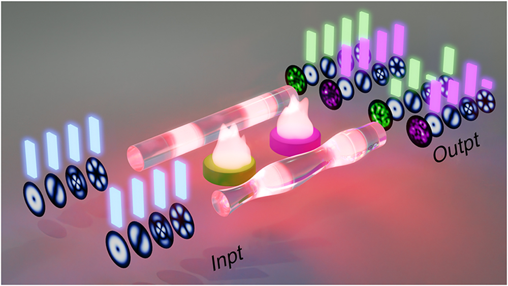
Fig. 1. Concept of spatially resolved sensing enabled by distributed mode mixing: comparison between a longitudinally invariant fiber and a fiber with diameter variations. The light within a multimode optical fiber consists of a superposition of eigenmodes, each carrying a portion of the total power propagating in the fiber. A perturbation on the fiber will induce mode-dependent phase changes, which will manifest as a change in the output of the fiber, whether this is the spatial interference pattern (specklegram) shown in the figure, or the wavelength domain interference spectrum used in this work. In this figure, two different longitudinal positions that experience identical perturbations are shown in green and purple, resulting in the corresponding color-coded modal amplitudes. For a perfectly longitudinally invariant fiber (left), the position of this perturbation will be indistinguishable at the output, as the modes will travel through the fiber free from coupling and power redistribution, thus rendering the effect of mode-dependent optical path length changes position-independent. In the case of an optical fiber with longitudinal variations (right), mode coupling leads to modal power redistribution, rendering the effect of these path length changes position-dependent, hence allowing for longitudinally resolved sensing.

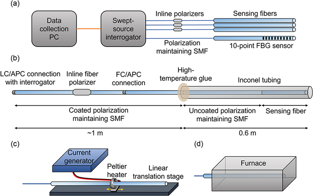
Fig. 2. Experimental setup. (a) Overview of the setup used to collect wavelength intensity spectra from the fibers under different temperature distributions. (b) Schematic and dimensions of the sensors. The length of sensing fiber for each of the sensors was 0.13 m for the sapphire fiber, 0.24 m for the suspended-core fiber, and 0.29 m for the graded-index fiber. The fibers were housed within Inconel tubing to shield them from potential contaminants that would burn at high temperatures. The tubing was sealed with high temperature glue at the proximal end and a crimp at the distal end. (c) Experimental setup for the localized heating experiment. (d) Experimental setup for the furnace heating experiment. The fibers were subjected to various temperature distributions by being placed in a furnace, with the distributions being varied by manually translating the fibers relative to the furnace and applying a range of furnace temperatures per sensor position.

Fig. 3. Variation in sapphire fiber diameter as a function of position for two samples of fiber, highlighting the variability. (a) This section was arbitrarily selected. (b) This section was selected as an extreme example of strong variation in diameter. The lengths of fiber were selected from the same, originally longer length of sapphire fiber, as used in the main experiment.

Fig. 4. Results from the localized heating experiment. (a) Average correlation coefficient of spectra collected during each 30 min heating position against the reference spectrum. (b) Heat distributions from the localized heating experiment, as taken using the FBG sensor. (c)–(e) Example spectra over a zoomed-in wavelength range from all five heating positions for the sapphire, suspended-core, and graded-index fiber, respectively.

Fig. 5. Heat distributions from the furnace heating experiment. Note that this is a representation of the axis along which the sensors were translated and the approximate relative sensor positions and is not to scale. (a)–(c) Temperature distributions from three different sensor positions. Within each plot/sensor position, the temperature distributions from three different furnace temperatures are shown.

Fig. 6. Predictions made by the DNNs on the 10-point temperature distributions from the test wavelength interference spectra. (a)–(c) show predictions made by the linear regressor. (d)–(f) show predictions made by the MLP. (a) and (d) show the predictions from DNNs trained on sapphire spectra, (b) and (e) SCF spectra, and (c) and (f) graded-index (GRIN) fiber spectra. (g) and (h) show the RMS error for (g) linear regressor and (h) multilayer perceptron for each sensing position along the three fibers.

Fig. 7. Deep neural network loss history. (a)–(c) Training (blue) and validation (red) mean-squared error (MSE) loss as a function of epoch for the MLP trained on (a) sapphire fiber spectra, (b) SCF spectra, and (c) graded-index (GRIN) fiber spectra. (d)–(f) Training and validation mean-squared error loss as a function of epoch for the linear regressor trained on (d) sapphire fiber spectra, (e) SCF spectra, and (f) GRIN fiber spectra.

Table 1. Comparison between the Three Sensing Fibers for a Few Relevant Properties, Including Cross-Sectional Image/Refractive Index Profile, Numerical Apertures, Core Diameters, and an Approximate Number of Supported Modes