Laser-driven inertial confinement fusion (ICF) is a feasible method to realize controllable fusion, which is expected to be one of the best solutions for the global energy problem^[1]. In a laser-driven ICF facility, several high-power coherent laser beams uniformly focus on a micro-dimension target to generate high-temperature and high-pressure conditions, thereby causing atomic fusion^[2]. Moreover, this method can also be used to explore basic sciences, such as astrophysics phenomena, materials science, nuclear science, and so on.

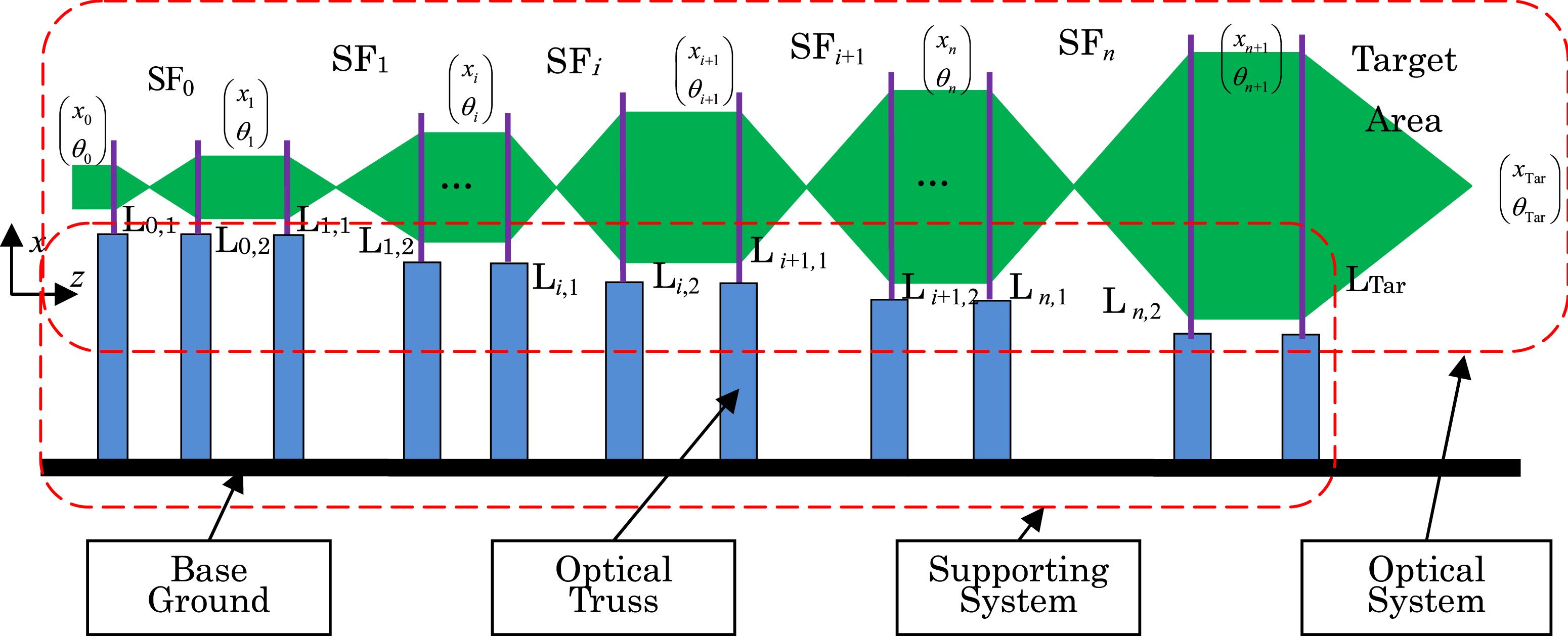
Each coherent laser beam initially transmits lots of optics for hundreds of meters to enhance its energy and adjust its proper direction to achieve the aforementioned conditions^[3]. A typical diagram of a single laser beam in a laser-driven ICF facility after removing all the mirrors is given in Figure 1. The laser beam is magnified by several spatial filters, and the whole optical system is supported by optical trusses fixed to the base ground. However, a tiny disturbance in the optics would affect the beam stability during its long-distance propagation and high precision. Thus, a laser-driven ICF facility requires extreme high precision. Furthermore, researchers have conducted excellent studies on the experimental environment surrounded by all kinds of vibration disturbances. For instance, Tietbohl et al.^[4] analyzed the beam stability caused by mirror supporting systems. Swensen et al.^[5] analyzed the errors caused by structural vibration using the finite element method. Liu et al.^[6,7] built a new structural model for analyzing the errors induced by structural vibrations and analyzed the lens vibration sensitivities to the ICF facility targets. Several optics exist in a laser-driven ICF facility; however, the same error on different optics would have different effects on the target, indicating that the error sensitivities to the target would be different with different optics.

This study focused on how the errors of different optics contributed to the target. The errors were mainly caused by vibrations, and thus were regarded as vibration sensitivities. Section 2 describes in detail the vibration sensitivities of the lenses and reflecting mirrors in a laser-driven ICF facility, including their features. In Section 3, we report how the theoretical models in Section 2 were applied to SG-II facilities, and the results that were obtained. Section 4 describes several practical mechanical structure designs to eliminate errors and decrease system errors.

There are mainly two kinds of vibration-sensitive optics in ICF facilities. One is the focusing lenses and the other is the reflecting mirrors. Previous studies indicated that only the translational movements of the lenses and the rotational disturbances affect the beam direction.

A schematic of the lenses for a single beam in laser-driven ICF facilities is shown in Figure 1. The two adjacent focusing lenses are initially combined to form a spatial filter to adjust the beam quality. Finally, the laser beam reaches the target area and is focused by the targeting lens ${\mathrm{L} }_{\mathrm{Tar} } $ after passing through several filters.

The lenses are forced to vibrate because of the disturbances. However, only translational disturbance should be discussed because the rotational vibration is insensitive to the beam direction. For simplicity, the discussion on the vibrating model is based on three hypotheses: the lenses vibrate around their ideal positions, indicating that their average displacements from the required place over time are zero; only the $x$-direction translational vibration was taken into account without loss of generality; and the targeting lens ${\mathrm{L} }_{\mathrm{Tar} } $ was relatively fixed, indicating that no positional error occurred between the two objects.

According to Ref. [7], the relationship between the incident beam into the $i\mathrm{th} $ spatial filter $({\mathrm{SF} }_{i} )$ and the $(i+ 1)\mathrm{th} $ spatial filter $({\mathrm{SF} }_{i+ 1} )$ satisfies (1)$$\displaystyle \left( \begin{array}{ @{}c@{}} \displaystyle {x}_{i+ 1} \\ \displaystyle {\theta }_{i+ 1} \\ \displaystyle 1\end{array} \right)= \left( \begin{array}{ @{}ccc@{}} \displaystyle - {m}_{i} & \displaystyle {k}_{i} & \displaystyle {r}_{i} \\ \displaystyle 0 & \displaystyle - \frac{1}{{m}_{i} } & \displaystyle {g}_{i} \\ \displaystyle 0 & \displaystyle 0 & \displaystyle 1\end{array} \right)\left( \begin{array}{ @{}c@{}} \displaystyle {x}_{i} \\ \displaystyle {\theta }_{i} \\ \displaystyle 1\end{array} \right)= \left[{B}_{i} \right]\left( \begin{array}{ @{}c@{}} \displaystyle {x}_{i} \\ \displaystyle {\theta }_{i} \\ \displaystyle 1\end{array} \right), \displaystyle$$(2)$$\displaystyle {m}_{i} = \frac{{f}_{i, 2} }{{f}_{i, 1} } = \frac{{D}_{i, 2} }{{D}_{i, 1} } , \displaystyle$$(3)$$\displaystyle {k}_{i} = {f}_{i, 1} + {f}_{i, 2} - \frac{{l}_{i} }{{m}_{i} } , \displaystyle$$(4)$$\displaystyle {r}_{i} = \left(1+ {m}_{i} + \frac{{l}_{i} }{{f}_{i, 2} } \right){a}_{i, 1} - \frac{{l}_{i} }{{f}_{i, 2} } {a}_{i, 2} , \displaystyle$$(5)$$\displaystyle {g}_{i} = \frac{{a}_{i, 1} - {a}_{i, 2} }{{f}_{i, 2} } , \displaystyle$$ where ${x}_{i} $ and ${\theta }_{i} $ are the displacement and the angle of incident beam into ${\mathrm{SF} }_{i} $, respectively; ${x}_{i+ 1} $ and ${\theta }_{i+ 1} $ are the displacement and the angle of incident beam into ${\mathrm{SF} }_{i+ 1} $, respectively; [${B}_{i} $] is the transfer matrix of ${\mathrm{SF} }_{i} $; ${D}_{i, 1} $ and ${D}_{i, 2} $ are the beam apertures in ${\mathrm{L} }_{i, 1} $ and ${\mathrm{L} }_{i, 2} $, respectively; ${m}_{i} $ is the beam aperture expanding ratio (BAER) in ${\mathrm{SF} }_{i} $; ${l}_{i} $ is the distance between the second lens of ${\mathrm{SF} }_{i} $ (${\mathrm{L} }_{i, 2} $) and the first lens of ${\mathrm{SF} }_{i+ 1} ({\mathrm{L} }_{i+ 1, 1} )$; ${f}_{i, 1} $ and ${f}_{i, 2} $ are the focal lengths of ${\mathrm{L} }_{i, 1} $ and ${\mathrm{L} }_{i, 2} $ in ${\mathrm{SF} }_{i} $, respectively; and ${a}_{i, 1} $ and ${a}_{i, 2} $ are the $x$-axis translational displacements of ${\mathrm{L} }_{i, 1} $ and ${\mathrm{L} }_{i, 2} $, respectively ^[7].

In the last part, the laser beam was focalized to the target by ${\mathrm{L} }_{\mathrm{Tar} } $, and the transfer matrix [C] from the incident beam into ${\mathrm{L} }_{\mathrm{Tar} } $ to the focal plane satisfies (6)$$[C] = \left( \begin{array}{ @{}ccc@{}} \displaystyle 0 & \displaystyle {f}_{T} & \displaystyle {a}_{T} \\ \displaystyle - \frac{1}{{f}_{T} } & \displaystyle 1 & \displaystyle \frac{{a}_{T} }{{f}_{T} } \\ \displaystyle 0 & \displaystyle 0 & \displaystyle 1\end{array} \right),$$ where ${f}_{T} $ is the focal length of ${\mathrm{L} }_{\mathrm{Tar} } $ and ${a}_{T} $ is the vibrating displacement of ${\mathrm{L} }_{\mathrm{Tar} } $.

Supposing $n+ 1$ spatial filters are marked from ${\mathrm{SF} }_{0} $ to ${\mathrm{SF} }_{n} $, and combining Equation (1) to Equation (6), the beam information on the target ${\left( \begin{array}{ @{}cc@{}} \displaystyle {x}_{\mathrm{Tar} } & \displaystyle {\theta }_{\mathrm{Tar} } \end{array} \right)}^{{}^{\prime } } $ then satisfies (7)$$\displaystyle {\left( \begin{array}{ @{}ccc@{}} \displaystyle {x}_{\mathrm{Tar} } & \displaystyle {\theta }_{\mathrm{Tar} } & \displaystyle 1\end{array} \right)}^{\prime } = [C] [{B}_{n} ] \cdots [{B}_{i} ] \cdots [{B}_{0} ] {\left( \begin{array}{ @{}ccc@{}} \displaystyle {x}_{0} & \displaystyle {\theta }_{0} & \displaystyle 1\end{array} \right)}^{\prime } , \displaystyle $$ where ${x}_{0} $ and ${\theta }_{0} $ are the displacement and the angle of the whole optical incident beam, respectively.

Finally, the position of the laser beam focalized in the focal plane ${x}_{\mathrm{Tar} } $ is (8)$$\begin{aligned}\displaystyle {x}_{\mathrm{Tar} } = &\displaystyle \frac{\mathop{(- 1)}\nolimits ^{n+ 1} }{\displaystyle \prod _{i= 0}^{n} {m}_{i} } {f}_{T} {\theta }_{0} + \sum _{i= 0}^{n} \mathop{(- 1)}\nolimits ^{n- i} {q}_{i} ({a}_{i, 1} - {a}_{i, 2} )\\ &\displaystyle + \hspace{0.167em} {a}_{T} ,\end{aligned}$$(9)$$\begin{aligned}\displaystyle {q}_{i} &= \displaystyle \frac{1}{\displaystyle \prod _{j= i}^{n+ 1} {m}_{j} } \frac{{f}_{T} }{{f}_{i, 1} } = \frac{1}{\displaystyle \prod _{j= i+ 1}^{n+ 1} {m}_{j} } \frac{{f}_{T} }{{f}_{i, 2} } = \frac{{D}_{i, 1} }{{D}_{T} } \frac{{f}_{T} }{{f}_{i, 1} } \\\displaystyle &= \displaystyle \frac{{D}_{i, 2} }{{D}_{T} } \frac{{f}_{T} }{{f}_{i, 2} } ,\end{aligned}$$ where ${D}_{\mathrm{T} } $ is the beam aperture in ${\mathrm{L} }_{\mathrm{Tar} } $. ${m}_{n+ 1} $ is set to zero when only $n+ 1$ spatial filters exist, to simplify the expression.

The transmissibility error from each vibrating lens to the target was defined as the lens vibration sensitivity (LVS); thus, the following equations were obtained according to Equations (8) and (9): (10)$$\displaystyle \Delta {x}_{i, 1} = \mathop{(- 1)}\nolimits ^{n- i} {q}_{i} {a}_{i, 1} (t)= \mathop{(- 1)}\nolimits ^{n- i} \frac{{D}_{i, 1} }{{D}_{T} } \frac{{f}_{\mathrm{T} } }{{f}_{i, 1} } {a}_{i, 1} (t), \displaystyle$$(11)$$\displaystyle \Delta {x}_{i, 2} = \mathop{(- 1)}\nolimits ^{n+ 1- i} {q}_{i} {a}_{i, 2} (t)= {\left(- 1\right)}^{n+ 1- i} \frac{{D}_{i, 2} }{{D}_{T} } \frac{{f}_{T} }{{f}_{i, 2} } {a}_{i, 2} (t). \displaystyle$$ The absolute LVS values of the two lenses in ${\mathrm{SF} }_{i} $ were both ${q}_{i} $, but they are opposite in direction. Based on Equations (10) and (11), the LVS is: (i)

proportional to the focal length of the focusing lens,

In ICF facilities, mirrors are widely used to change beam directions. Based on the placement, mirrors are classified into two circumstances: in the first, the mirrors are placed in the spatial filters, and in the second, they are between the spatial filters.

A schematic of a mirror placed in the $i\mathrm{th} $ spatial filter is given in Figure 2. The reflecting mirror M is placed between ${\mathrm{L} }_{i, 1} $ and ${\mathrm{L} }_{i, 2} $ in ${\mathrm{SF} }_{i} $, Ideally, the reflecting mirror M is in state 1, and the central-dashed line S0–S–S1 is the ideal beam path from ${\mathrm{L} }_{i, 1} $ to ${\mathrm{L} }_{i, 2} $. However, for some reason, the reflecting mirror M changed to state 2 with an angle of $\Delta {\theta }_{i} $, and the real beam path was changed to S0–S–S2, marked with the solid line after the reflecting mirror M. By calculation, the emergent beam was deflected by $2\Delta {\theta }_{i} $. The equivalent schematic is shown in Figure 2b.

Supposing the beam deflection was generated by the deviation of ${\mathrm{L} }_{i, 1} $, the deviation of ${\mathrm{L} }_{i, 1} $ was calculated as $2\Delta {\theta }_{i} {f}_{i, 1} $^[8]. In other words, the error effect of the reflecting mirror in ${\mathrm{SF} }_{i} $ to the target with an angular deflection of $\Delta {\theta }_{i} $ was equivalent to the error generated by ${\mathrm{L} }_{i} $ in ${\mathrm{SF} }_{i} $, with a translational deviation of $2\Delta {\theta }_{i} {f}_{i, 1} $.

Based on Equation (10), the error in the target $\Delta {x}_{1i} $ generated by the reflecting mirror in ${\mathrm{SF} }_{i} $, with deflection of $\Delta {\theta }_{i} $ is (12)$$\displaystyle \Delta {x}_{1i} = \mathop{(- 1)}\nolimits ^{n- i} {p}_{1i} \Delta {\theta }_{i} , \displaystyle$$(13)$$\displaystyle {p}_{1i} = \frac{2{f}_{T} }{\displaystyle \prod _{j= i}^{n+ 1} {m}_{j} } = 2{f}_{T} \frac{{D}_{i, 1} }{{D}_{T} } , \displaystyle$$ where ${p}_{1i} $ is regarded as the mirror vibration sensitivity (MVS) of the reflecting mirrors in ${\mathrm{SF} }_{i} $, since the MVS represents the transmissibility error from the reflecting mirror to the target.

Supposing the mirror is placed between ${\mathrm{SF} }_{i- 1} $ and ${\mathrm{SF} }_{i} $, similar to the mirrors in spatial filters, the lenses in Figure 2 should be replaced, so ${\mathrm{L} }_{i, 1} $ and ${\mathrm{L} }_{i, 2} $ are replaced by ${\mathrm{L} }_{i- 1, 2} $ and ${\mathrm{L} }_{i, 1} $. Similarly, the error in target $\Delta {x}_{2i} $ generated by the reflecting mirror between ${\mathrm{SF} }_{i, 1} $ and ${\mathrm{SF} }_{i} $ with deflection of $\Delta {\theta }_{i} $ satisfies (14)$$\displaystyle \Delta {x}_{2i} = \mathop{(- 1)}\nolimits ^{n- i} {p}_{2i} \Delta {\theta }_{i} , \displaystyle$$(15)$$\displaystyle {p}_{2i} = \frac{2{f}_{T} }{\displaystyle \prod _{j= i}^{n+ 1} {m}_{j} } = 2{f}_{T} \frac{{D}_{i- 1, 2} }{{D}_{T} } = 2{f}_{T} \frac{{D}_{i, 1} }{{D}_{\mathrm{T} } } , \displaystyle$$ where ${p}_{2i} $ is the MVS of the reflecting mirrors between ${\mathrm{SF} }_{i, 1} $ and ${\mathrm{SF} }_{i} $.

The MVS values (${p}_{T} $) between the last spatial filter and the target can also be included in this expression by regarding the beam aperture as ${D}_{\mathrm{T} } $.

The comparison between Equations (14) and (15) and Equations (12) and (13) shows that the MVS values of the mirrors between the spatial filters were the same as those of the mirrors between the spatial filter and the preceding spatial filter.

The MVS values of the reflecting mirrors in the spatial filters and the reflecting mirrors between the spatial filter and its preceding spatial filter are all expressed as ${p}_{i} $ to simplify the expression. The subscript $i$ represents the $i\mathrm{th} $ spatial filter, thereby obtaining the following equation: (16)$${p}_{i} = {p}_{1i} = {p}_{2i} = \frac{2{f}_{T} }{\displaystyle \prod _{j= i}^{n+ 1} {m}_{j} } = 2{f}_{T} \frac{{D}_{i, 1} }{{D}_{T} } .$$

Based on Equation (16), the MVS is (i)

proportional to the focal length of the focusing lens, and

Generally, the disturbances on optics can be attributed into two forms: one is ground vibrations and the other is air turbulence or the acoustic vibrations. In the first case, ground vibrations are transmitted to the optics via the optical trusses, which are mainly made of steel. In the second case, acoustic vibrations directly act on the optics via air. Furthermore, ground vibrations and air turbulence arise from several sources, such as traffic, people working, air compressors, air conditioners, motors, people talking, loudspeakers, and so on.

Several vibrating sources and vibration-sensitive optics exist; thus, normal distribution was utilized to evaluate the system error. Based on Equation (10) to Equation (16), the variance generated by the lenses and mirrors is (17)$$\displaystyle { \Delta }_{L}^{2} = \sum _{i= 0}^{n} q_{i}^{2} (\Delta _{\mathrm{L} i, 1}^{2} + \Delta _{Li, 2}^{2} )+ \Delta _{T}^{2} , \displaystyle$$(18)$$\displaystyle { \Delta }_{M}^{2} = \sum _{i= 0}^{n} \left(p_{i}^{2} \sum _{j= 0}^{{u}_{i} } \Delta _{Mi, j}^{2} \right)+ \sum _{j= 0}^{{w}_{\mathrm{T} } } p_{T}^{2} \Delta _{{}_{MT, j} }^{2} , \displaystyle$$(19)$$\displaystyle { \Delta }_{Mi, 0}^{2} = 0, \displaystyle$$(20)$$\displaystyle { \Delta }_{MT, 0}^{2} = 0, \displaystyle$$ where ${ \Delta }_{L}^{2} $ is the total variance in the target generated by the lenses in the spatial filters; ${ \Delta }_{M}^{2} $ is the total variance in the target generated by the reflecting mirrors; ${ \Delta }_{Li, 1}^{2} $ and ${ \Delta }_{Li, 2}^{2} $ are the variances of the two lenses in ${\mathrm{SF} }_{i} $, respectively; ${ \Delta }_{T}^{2} $ is the variance of the focusing lens; ${u}_{i} $ is the numbers of the reflecting mirrors between ${\mathrm{SF} }_{i, 1} $ and ${\mathrm{SF} }_{i} $ in ${\mathrm{SF} }_{i} $; ${ \Delta }_{{}_{Mi, j} }^{2} $ is the mean variance of the $j\mathrm{th} $ of the ${u}_{i} $ reflecting mirrors; and ${ \Delta }_{MT, j}^{2} $ is the variance of the $j\mathrm{th} $ of the ${w}_{T} $ reflecting mirrors between the last spatial filter and the focusing lens.

Based on Equation (17), the variations of the two lenses in ${\mathrm{SF} }_{i} $ have the same impact on the target variation, with a factor of ${ q}_{i}^{2} $. Thus, ${ q}_{i}^{2} $ is defined as the spatial filter lens variation weight factor (SFLVWF). Similarly, in Equation (18), ${ p}_{i}^{2} $ is defined as the spatial filter mirror variation weight factor (SFMVWF). The SFLVWFs and SFMVWFs in a laser-driven ICF facility are illustrated in Figure 3.

The SG-II facility is currently composed of three sub-facilities, namely, SG-II Origin, SG-II Additional beam, and SG-II Updated. The previous two facilities use two-pass amplification (TPA) technology, whereas the updated facility uses four-pass amplification (FPA) technology. The TPA or FPA systems were considered as two or four spatial filters, respectively, to analyze the facilities based on the theory in the previous section. In addition, the optical system parameters of the three SG-II facilities are listed in Tables 1–3.

The SFLVWFs of the three facilities are shown in Figure 4. Comparing the SFLVWFs in the three facilities, the following conclusions were obtained.

(i)

The most vibration-sensitive spatial filters in SG-II Origin and SG-II Additional beam were ${\mathrm{SF} }_{6} $ and ${\mathrm{SF} }_{7} $, respectively.

The SFMVWFs in the three facilities are shown in Figure 5, from which the following conclusions were obtained. (i)

The SFMVWFs grew gradually with decreasing distance to the target in SG-II Origin and SG-II Additional beam because the beam apertures were magnified step by step in the two facilities.

Compared with the other two facilities, SG-II Updated with the FPA system leveled the SFLVWFs in the FPA system and increased the numbers of sensitive mirrors. The parameters of the FPA system were changed for comparison with the real parameters to find out the features of the FPA system in terms of vibration sensitivities. The parameters are listed in Table 4, and the results are shown in Figures 6–8. The results indicated the following. (i)

The SFLVWFs in FPA system were the same.

As was discussed in the previous two sections in detail, the sensitivities of the optics in laser-driven ICF facilities vary according to the optical parameters. Thus, the appropriate optical parameters that would efficiently enhance the stability of the system should be chosen. Based on Equations (9) and (16), it would be better if:

(i)

the focal lengths of the focusing lens was shorter,

Another method to enhance the beam positioning stability is to eliminate the vibration sources, which can be done in two ways: decreasing the mechanical vibration responses and preventing error accumulation. In SG-II facilities, the following methods were utilized.

(i)

Some modules were isolated from other modules, as shown in Figure 8.

This study aimed at stabilizing the beams in laser-driven ICF facilities. The errors on each of optics make different contributions to the targeting stability, and thus, an efficient solution for stabilizing the beams has to eliminate the errors on error-sensitive optics. Therefore, the vibration sensitivities of each optic were initially obtained. The vibration-sensitive optics should be given more attention to enhance the dynamic beam stabilities from the mechanical point of view. The comparison among the three ICF facilities of SG-II indicated that the SG-II Updated facility was the most vibration-sensitive facility because the FPA technology increased the SFMVWFs in the FPA system.

This study also pointed out that decreasing the focal length of the focusing lens, increasing the focal lengths of the lenses in the spatial filters, and enlarging the total BAER would decrease the vibration sensitivities of the optics. Moreover, a practical mechanical system design to decrease the beam errors including isolating the vibrating parts and enhancing the precision of target positioning and bound beams to prevent error accumulation must be employed to decrease the impact of vibrations on the optical system.