
Feng Jinchao, Chang Di, Li Zhe, Sun Zhonghua, Jia Kebin. Cherenkov-Excited Luminescence Scanned Tomography Reconstruction Based on Approximate Message Passing[J]. Chinese Journal of Lasers, 2020, 47(2): 207027
- Chinese Journal of Lasers
- Vol. 47, Issue 2, 207027 (2020)
![Diagram of CELSI[3]. (a) CELSI imaging instrument; (b) process of photon excitation](/richHtml/zgjg/2020/47/2/0207027/img_1.jpg)
Fig. 1. Diagram of CELSI[3]. (a) CELSI imaging instrument; (b) process of photon excitation
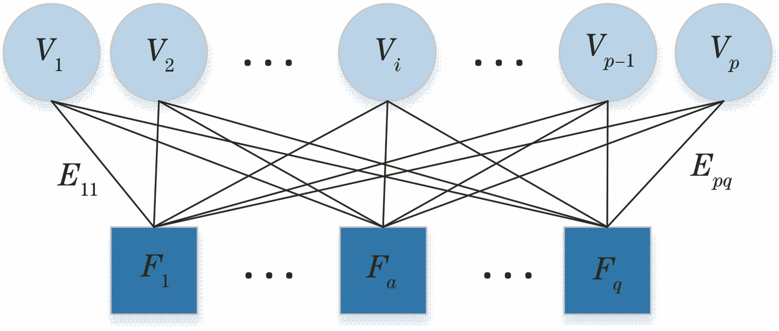
Fig. 2. Structure of completely bipartite factor graph
Fig. 3. Flow chart of AMP algorithm
Fig. 4. Phantom used in experiments
Fig. 5. Reconstructed images obtained by different algorithms with varied contrasts. Contrast of Figs. 5(a)--(f) is reduced from 4 to 1.5 by step of 0.5
Fig. 6. Profiles along horizontal line of reconstructed images of single target. (a) Contrast is 4; (b) contrast is 3; (c) contrast is 2
Fig. 7. Distributions of true single targets with different radii and reconstruction results obtained by different algorithms. (a)--(e) Radius of fluorescent target decreases from 7 mm to 3 mm with a step of 1 mm
Fig. 8. Comparison of results obtained by different reconstruction methods for single targets with varied radius. (a) CNR; (b) MSE
Fig. 9. Reconstruction results of different algorithms for multiple fluorescent targets
|
Table 1. Background optical parameters of phantommm-1
| |||||||||||||||||||||||||||||||||||||||||||||||||||||||||||||||||||||||||||||||||||||||||||||||||||||||
Table 2. Quantitative comparison of reconstruction results obtained by three different methods (Tikhonov, ISTA, and AMP) with varied contrast
| ||||||||||||||||||||||||||||||||||
Table 3. Reconstruction time for different algorithms with varied contrasts
| ||||||||||||||||||||||||||||||||||||||||||||||||||||||||||||||||||||||||||||||||||||||
Table 4. Quantitative reconstruction results obtained by different algorithms for multiple fluorescent targets

Set citation alerts for the article
Please enter your email address
© Copyright 2018-2021 | Chinese Laser Press. All Rights Reserved 沪ICP备15018463号-20