
Tingting Gu, Haitao Zhao, Shaoyuan Sun. Depth Estimation of Single Infrared Image Based on Interframe Information Extraction[J]. Laser & Optoelectronics Progress, 2018, 55(6): 061010
- Laser & Optoelectronics Progress
- Vol. 55, Issue 6, 061010 (2018)
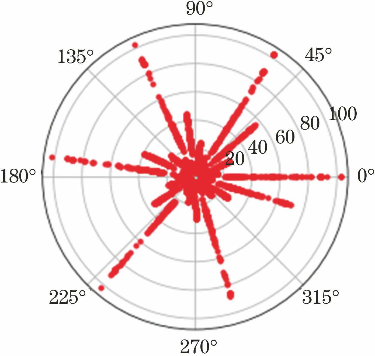
Fig. 1. Radar scatter plot
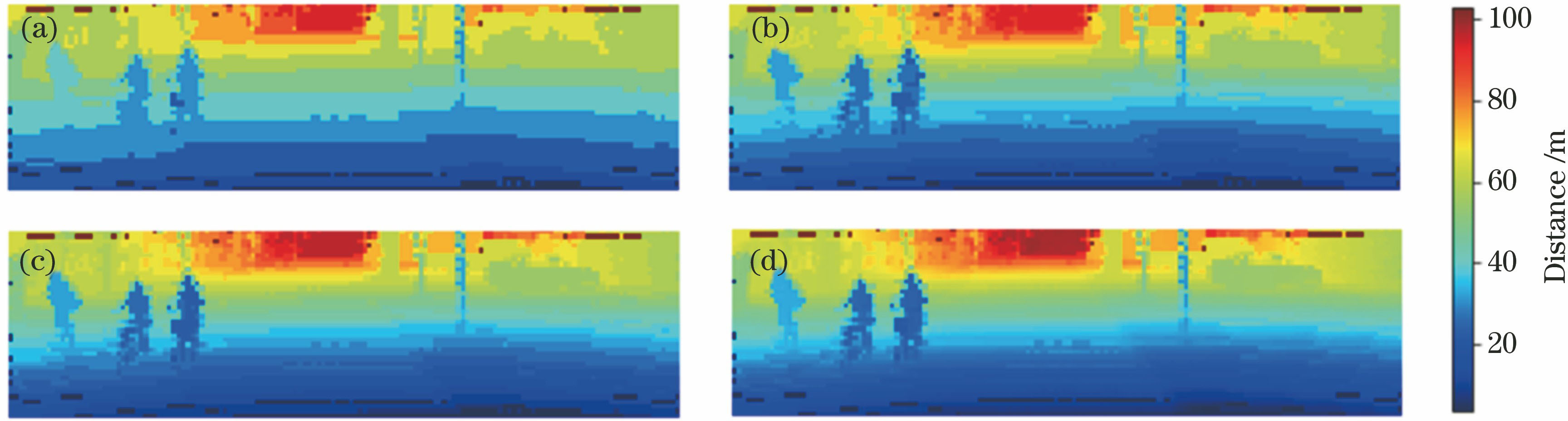
Fig. 2. Hierarchies of the ground truth. (a) 12 hierarchies; (b) 22 hierarchies; (c) 32 hierarchies; (d) original ground truth
Fig. 3. Architecture of proposed network
Fig. 4. Comparison of (a) 2D convolution and (b) 3D convolution
Fig. 5. Data acquisition equipment
Fig. 6. Infrared imaging and radar scatter plot at corresponding time. (a) Infrared imaging; (b) radar scatter points
Fig. 7. Comparison of traditional methods. (a) Scenario1; (b) scenario2; (c) scenario3; (d) scenario4
Fig. 8. Comparison of proposed method with traditional methods
Fig. 9. Data joint distribution. (a) Scenario1; (b) scenario2; (c) scenario3; (d) scenario4
Fig. 10. Comparison of experimental results. (a) Scenario1; (b) scenario2; (c) scenario3; (d) scenario4
|
Table 1. Convolutional kernel stride of 2D network residual blocks
|
Table 2. Architecture of 3D network
|
Table 3. Performance evaluation of comparative experiments

Set citation alerts for the article
Please enter your email address
© Copyright 2018-2021 | Chinese Laser Press. All Rights Reserved 沪ICP备15018463号-20