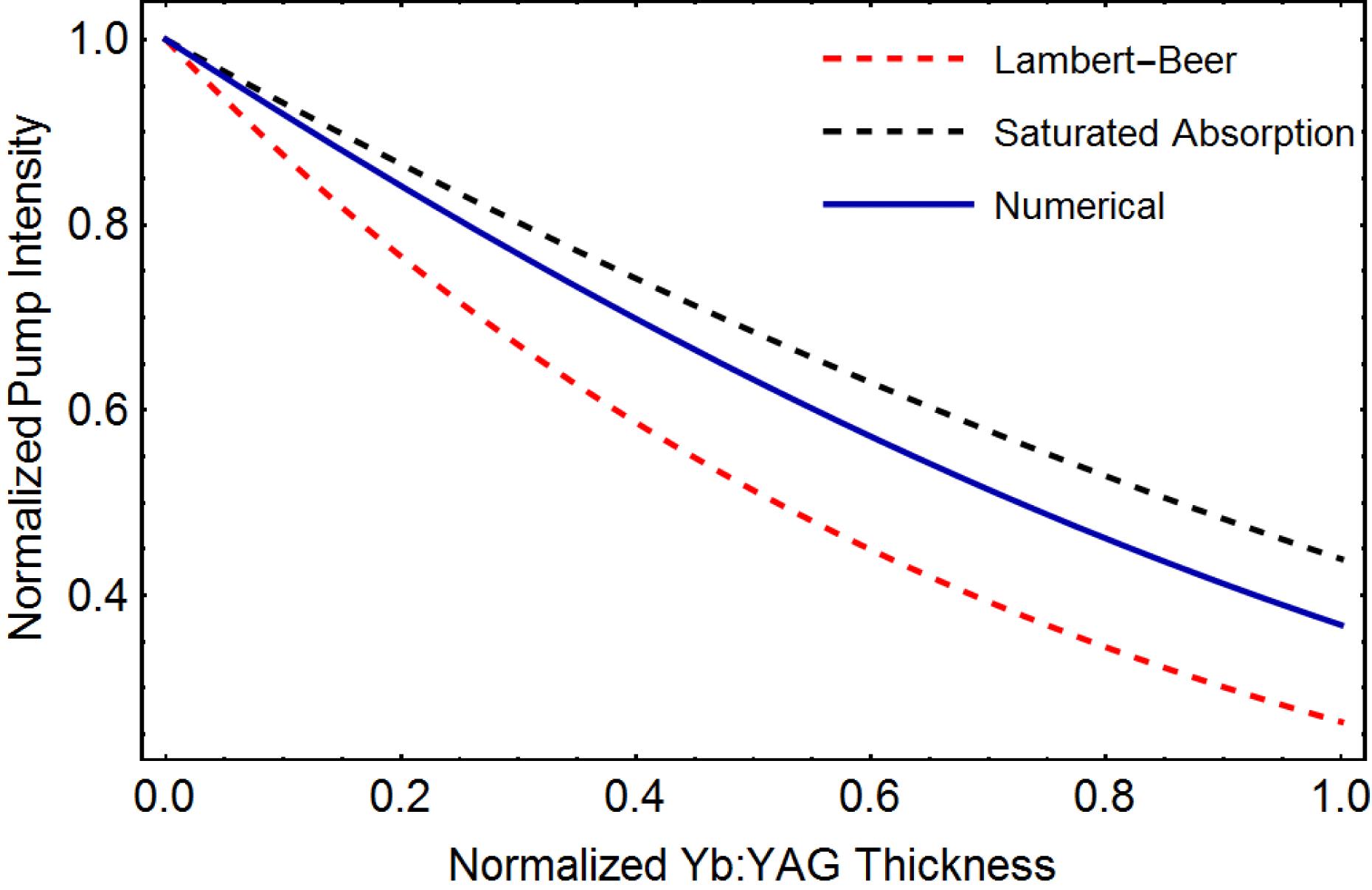

Issa Tamer, Sebastian Keppler, Jörg Körner, Marco Hornung, Marco Hellwing, Frank Schorcht, Joachim Hein, Malte C. Kaluza. Modeling of the 3D spatio-temporal thermal profile of joule-class  -based laser amplifiers[J]. High Power Laser Science and Engineering, 2019, 7(3): 03000e42
 -based laser amplifiers[J]. High Power Laser Science and Engineering, 2019, 7(3): 03000e42