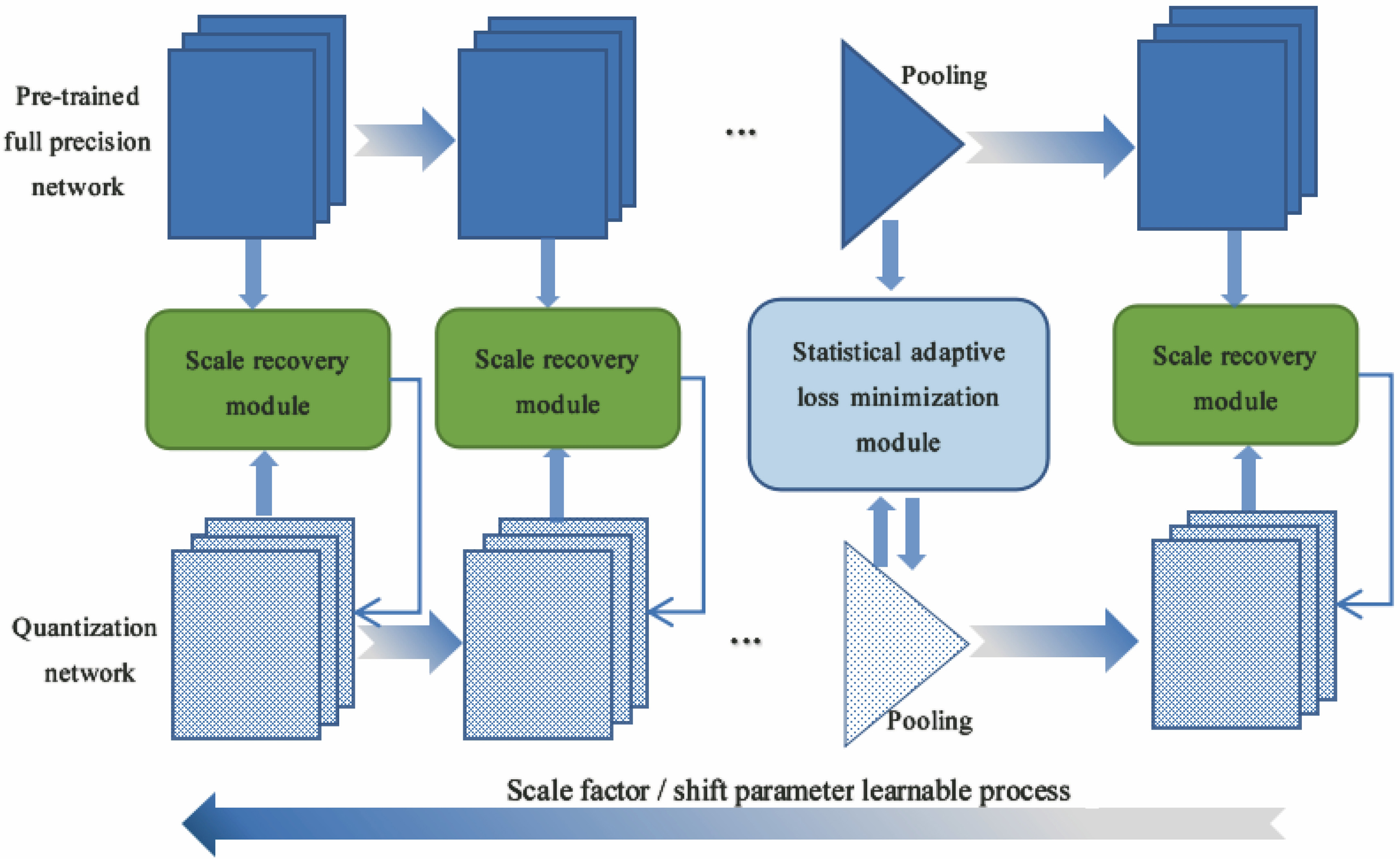
Fig. 1. General framework for point cloud learnable binary quantization network model

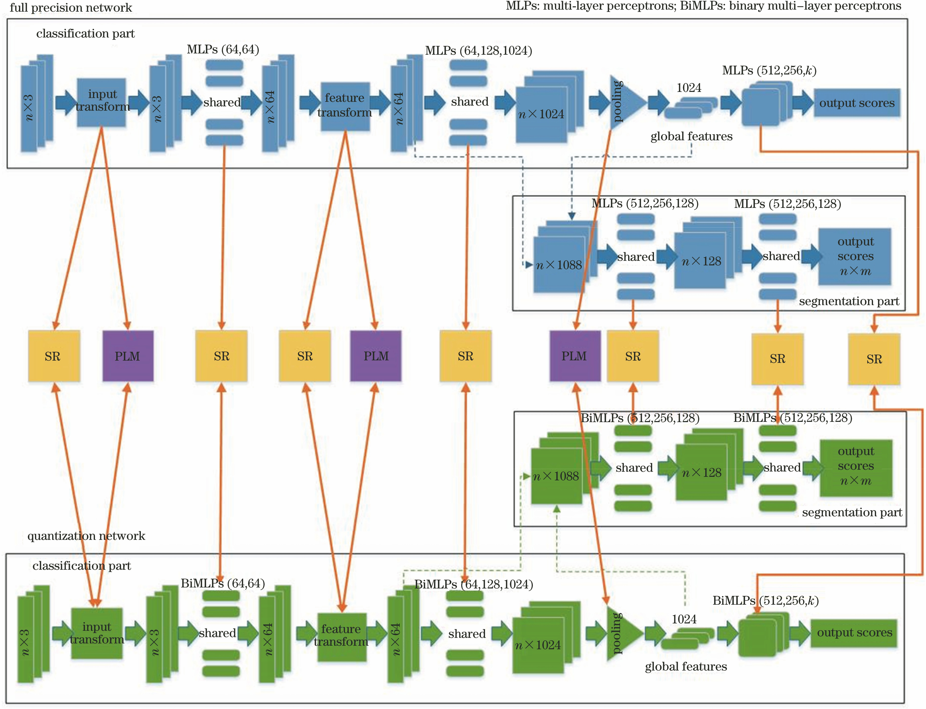
Fig. 2. Learnable binary quantization network model of PointNet

Fig. 3. Gene-algorithm based binary quantization scale factor recovery

Fig. 4. Optimal search of scale factor based on gene-algorithm optimization

Fig. 5. Curves of feature entropy before and after pooling. (a) n=5; (b) n=20; (c) n=50; (d) n=100

Fig. 6. Minimization of statistically self-adaptive pooling loss. (a) Quantitative network self-regulation; (b) statistical knowledge transfer regulation of full precision network

Fig. 7. Comparison of adjusted feature probability distributions. (a) Feature distribution comparison 1; (b) feature distribution comparison 2; (c) feature distribution comparison 3

Fig. 8. Learnable training process

Fig. 9. Comparison of optimized pooling. (a) Quantization network self-adjustment; (b) full-precision network transfer adjustment

Fig. 10. Training performance comparison. (a) Comparison result 1; (b) comparison result 2; (c) comparison result 3

Fig. 11. Scaling factor searching based on gene-optimized algorithm. (a) Iterative searching process; (b) feature maps produced by binary conv layer

Fig. 12. Comparison of different channel feature maps of different binary convolution layers (sub-figures from left to right are 3 corresponding channels in sequence). (a) Feature maps of different channels of 1^st binary convolution layer; (b) feature maps of different channels of 2^nd binary convolution layer; (c) feature maps of different channels of 3^rd binary convolution layer

Fig. 13. Comparison of feature maps of binary convolution layers at different locations (sub-figures from left to right are 3 convolution layers in sequence). (a) Feature map of location 1; (b) feature map of location 2; (c) feature map of location 3

Fig. 14. Feature maps of pooling. (a) Activation features before pooling; (b) pooling features of non-optimized binary network; (c) pooling features of binary network with pooling optimization; (d) pooling features of binary network with scaling and pooling optimization

Fig. 15. Partial results of part segmentation. (a) Knife; (b) motorbike; (c) lamp

Fig. 16. Partial results of semantic segmentation. (a) Area 1_Conference Room 2; (b) Area 1_Office Room 2; (c) Area 1_Hallway 1

Fig. 17. Overall performance comparisons. (a) Performance comparison 1; (b) performance comparison 2

Fig. 18. Inference time comparisons

Table 1. Comparison of binary quantization algorithms

Table 2. Comparison of binary quantization methods without optimized pooling

Table 3. Comparison of binary quantization methods with optimized pooling

Table 4. Comparison of typical binary quantization methods

Table 5. Precision of part segmentation%

Table 6. Semantic segmentation experiment results%

Table 7. Comparative experiment results for typical network models

Table 8. Complexity comparison results