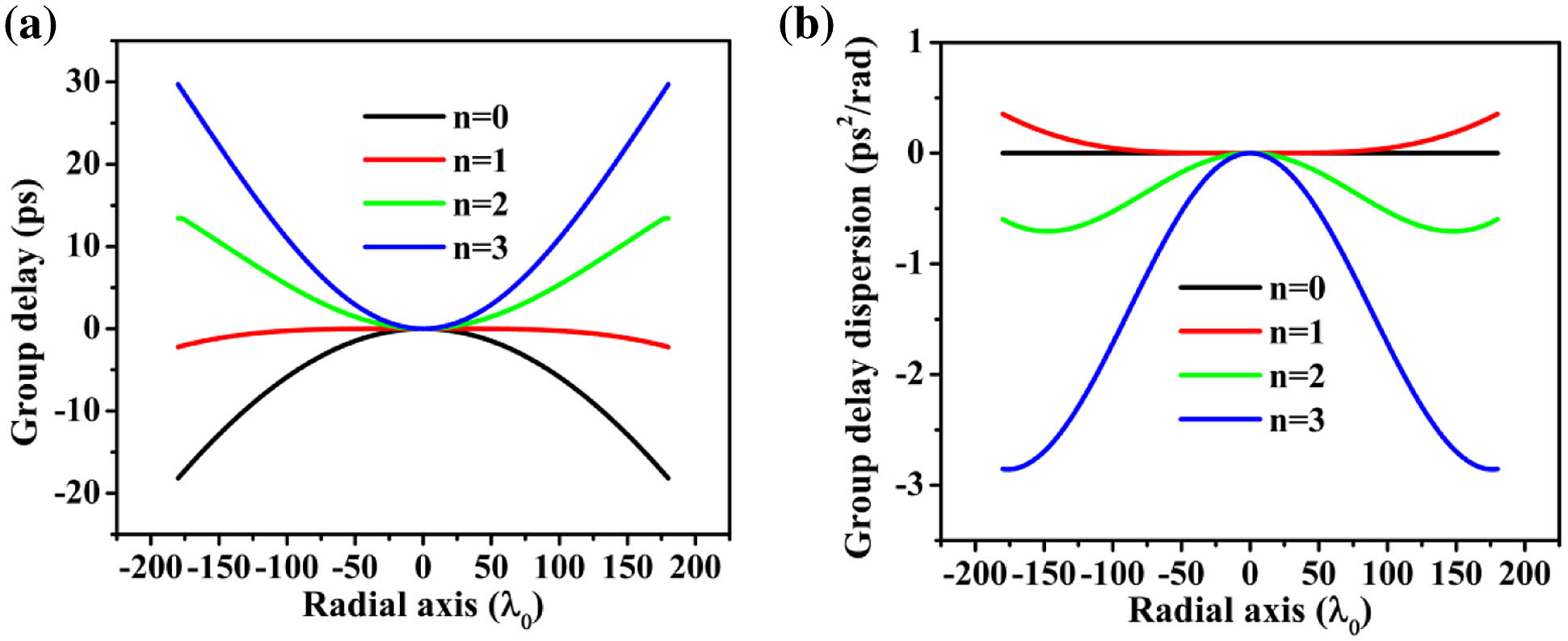
Fig. 1. Required relative (a) group delay and (b) group delay dispersion as a function of metalenses’ coordinates for different orders (n=0, 1, 2, and 3) of dispersion engineering. All curves are plotted based on Eqs. (3) and (4) for lenses with a focal length of 330λ0 at the designed wavelength and a radius of 180λ0.

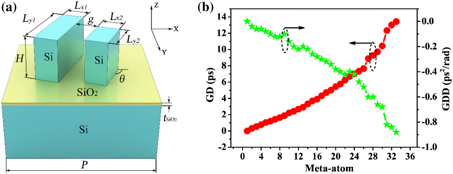
Fig. 2. (a) Schematic structure of the proposed dispersive meta-atom. The meta-atom consists of two Si blocks on a Si substrate with a SiO2 isolation layer, and the thickness of the SiO2 layer is tSiO2=2⁢ μm. (b) Relative group delay (GD) and group delay dispersion (GDD) of the 33 optimized meta-atoms.

Fig. 3. (a) Phase profile of the proposed hyper-dispersive metalens at the designed wavelength of λ0=118.8  μm, where the red curve is the ideal hyperbolic phase distribution along the radial direction, and the red squares denote the actual discrete phase distribution. (b) Amplitude transmittance distribution along the radial direction at the designed wavelength. (c) GD of the proposed hyper-dispersive metalens. The red solid curve is the ideal GD, and the blue dots are actual GD provided by the 33 optimized meta-atoms. (d) GDD of the proposed hyper-dispersive metalens. The green solid curve is the ideal GDD, and the navy dots are actual GDD provided by the 33 optimized meta-atoms.

Fig. 4. Intensity distribution of focused optical field in the x−z plane at six different optical frequencies, i.e., 2.40, 2.44, 2.48, 2.52, 2.56, and 2.61 THz for (a) hyper-dispersive metalens with actual GD and GDD, (b) hyper-dispersive metalens with ideal GD and GDD, and (c) regular diffractive metalens.

Fig. 5. (a) Optical intensity along the z axis at six different frequencies, i.e., 2.40, 2.44, 2.48, 2.52, 2.56, and 2.61 THz for the hyper-dispersive metalens with actual GD and GDD (top), hyper-dispersive metalens with ideal GD and GDD (middle), and regular diffractive metalens (bottom). (b) Normalized focal length shift (top), depth of focus (middle), and FWHM (middle) as a function of optical frequency for hyper-dispersive metalenses and regular diffractive metalens. The dashed line gives the corresponding diffraction limit. The bottom panel of (b) plots the focal length as a function of square angular frequency for hyper-dispersive metalenses.

Fig. 6. (a) Image of the fabricated hyper-dispersive metalens. (b) Zoom-in image of the area marked by the red square in (a).

Fig. 7. (a) Emission spectra of the THz QCL at drive current of 950 mA. (b) Experimental setup for the hyper-dispersive metalens, where the homemade THz blazed grating is used to select illuminating wavelength from broadband laser emission by changing its rotation angle.

Fig. 8. Measured focused optical field at different frequencies of 2.52, 2.54, 2.56, 2.58, and 2.60 THz. (a) Normalized two-dimensional intensity distribution on the x−z plane. (b) Normalized two-dimensional intensity distribution on the focal planes, as marked by the dashed lines. (c) Intensity distribution along the z axis. (d) Intensity distribution along the x direction (blue) and y direction (red) crossing the centers of the focal spots, where FWHMx and FWHMy give the sizes of the focal spot in the x and y directions.

Fig. 9. (a) Emission spectra of the QCL working at 650 and 950 mA. (b) Measured optical intensity distributions along the propagation direction at different currents. (c) Optical intensity distributions on the actual focal plane (yellow dashed line). (d) Intensity distribution curves in the x and y directions crossing the centers of the spots in (c).

Fig. 10. Comparison between experimental and simulation results. (a) Measured focal length (red dots) is plotted against the optical frequency along with its simulation (red triangles) counterparts, and the normalized focal length shift Δf is plotted as a function of the frequency for experimental (blue stars) and simulation (blue circles) results. (b) Measured (red dots) depth of focus is plotted against the optical frequency, and its simulation result (red triangles) is presented for comparison. The focal spot sizes in the x (blue stars) and y (blue triangles) directions are given at frequencies of 2.52, 2.54, 2.56, 2.58, and 2.60 THz, and the simulated result (blue squares) is also plotted for comparison. The pink dashed line denotes the diffraction limit.

Table 1. Major Parameters of Optimized Meta-Atoms (All Geometric Sizes are Given in Micrometers)