
Hua Zhong, Shiqi Xia, Yiqi Zhang, Yongdong Li, Daohong Song, Chunliang Liu, Zhigang Chen. Nonlinear topological valley Hall edge states arising from type-II Dirac cones[J]. Advanced Photonics, 2021, 3(5): 056001
- Advanced Photonics
- Vol. 3, Issue 5, 056001 (2021)
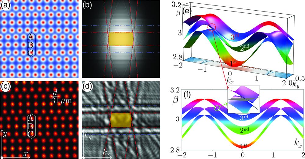
Fig. 1. Photonic lattices with type-II Dirac cones. (a) Numerically designed lattice structure with
![Linear topological VHE states at the DW between two type-II Dirac cone photonic lattices. (a) and (b) Inversion-symmetry-broken photonic lattices with the depth of site C and site A increased, respectively. (c) Band structure corresponding to the lattice in (a) [which looks the same for the lattice in (b)]. (d) Berry curvature of the first band displayed in the (kx,ky) plane. The top panel corresponds to (a); the bottom panel, which is opposite, corresponds to (b). The dashed hexagon represents the first BZ. (e) A DW is established by combining (a) and (b) with an interface, highlighted by a green rectangle. The lattice is periodic along the x direction but has boundaries along the y direction. (f) Band structure of the lattice in (e); the red curve represents the topologically protected VHE state along the DW. In panels (a), (b), and (e), blue and red spots represent the lattice sites with different detunings.](/richHtml/ap/2021/3/5/056001/img_002.png)
Fig. 2. Linear topological VHE states at the DW between two type-II Dirac cone photonic lattices. (a) and (b) Inversion-symmetry-broken photonic lattices with the depth of site C and site A increased, respectively. (c) Band structure corresponding to the lattice in (a) [which looks the same for the lattice in (b)]. (d) Berry curvature of the first band displayed in the
Fig. 3. Numerically obtained nonlinear topological VHE states and robust transport of quasi-solitons from MI. (a) Dispersion spectrum of the linear edge state in Fig. 2(f) . Solid curve is for
Fig. 4. Experimental observation of nonlinear topological VHE states. (a1) Experimentally established type-II Dirac lattices with a center DW (marked by the white line), where the inset (bottom-right) shows discrete diffraction from single-site excitation. (b)–(d) Linear (first and third rows) and nonlinear (second and fourth rows) outputs in real (first and second rows) and momentum (third and fourth rows) space obtained from excitation by two superimposed out-of-phase elliptical beams (circled by the dashed ellipse). The initial Bloch momenta of the probe beam are (b)

Set citation alerts for the article
Please enter your email address
© Copyright 2018-2021 | Chinese Laser Press. All Rights Reserved 沪ICP备15018463号-20