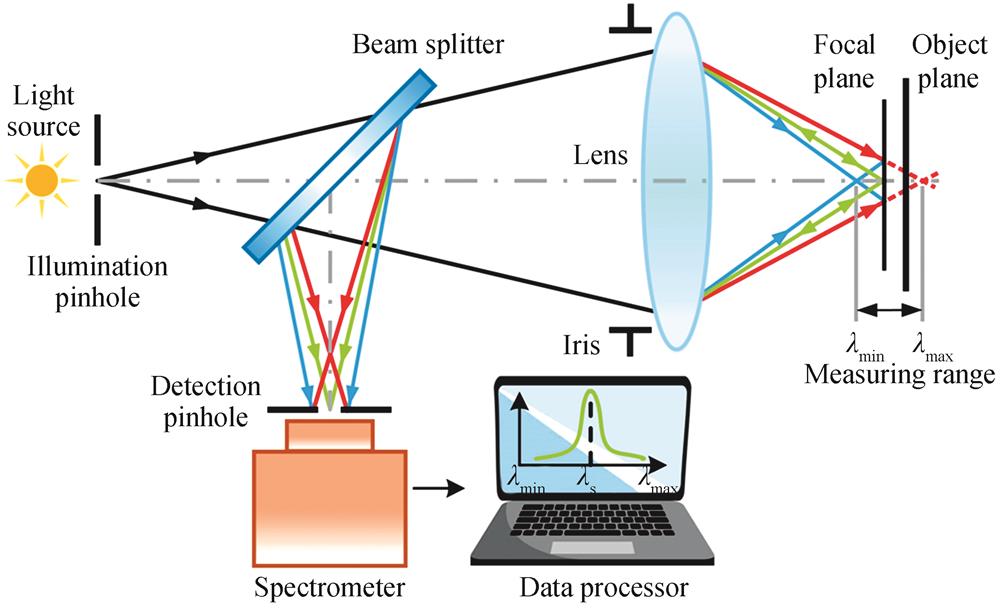
Fig. 1. Schematic of chromatic confocal measurement principle
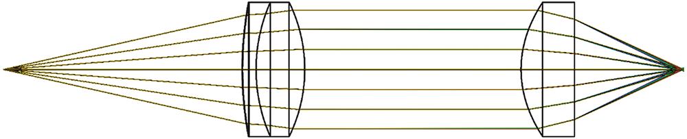
Fig. 2. Diagram of chromatic lens group
Fig. 3. Dispersion focal shift curve
Fig. 4. Chromatic confocal 3D measurement system
Fig. 5. Graphical user interface of the measurement software
Fig. 6. Optical path of chromatic confocal axial calibration experiment
Fig. 7. Comparison of four peak wavelength extraction algorithms
Fig. 8. 6-order polynomial fitting result of calibration curve
Fig. 9. Linear measurement interval of calibration curve
Fig. 10. Cubic spline interpolation of calibration curve
Fig. 11. Spectral data and peak extraction results of different algorithms
Fig. 12. Relative deviation of each position under different peak wavelength extraction algorithms(2 μm step)
Fig. 13. Axial resolution test results by fitting calibration method
Fig. 14. Axial resolution test results by interpolation calibration method
Fig. 15. Measurement result of a feeler step
Fig. 16. 3D profile measurement of flexible electrode
Fig. 17. 3D profile measurement of MEMS sample
Fig. 18. Thickness compensation model
[25] Fig. 19. Relationship between angle and wavelength
Component | Parameter |
---|
Light source | Wave band:400~800 nm | Fiber coupler | Diameter:50 μm multimode fiber,NA=0.22,50∶50 split ratio,Wave band:400~900 nm | Spectrometer | Resolution:0.7 nm,Wave band:200~1 100 nm |
|
Table 1. Main component parameters
Lens surface | Surface type | Curvature radius/mm | Thickness/mm | Optical glass | Semiaperture/mm |
---|
OBJ | Standard surface | ∞ | 44.120 | - | 0.000 | 1 | Even-order aspheric surface | 63.000 | 0.060 | 1.52,52.0 | 12.500 | 2 | Standard surface | 66.000 | 2.500 | S⁃TIH13 | 12.500 | 3 | Standard surface | 31.000 | 9.000 | S⁃FSL5 | 12.500 | 4 | Standard surface | -28.500 | 40.000 | - | 12.500 | 5 | Even-order aspheric surface | 20.130 | 9.857 | N-SF6 | 12.500 | 6 | Standard surface | ∞ | 18.979 | - | 12.500 | IMA | Standard surface | ∞ | - | - | 0.569 |
|
Table 2. Parameters of chromatic lens group
Polynomial order | 1 | 2 | 3 | 4 | 5 | 6 | 7 | 8 |
---|
R⁃square | 0.977 8 | 0.999 5 | 1 | 1 | 1 | 1 | 1 | 1 | RMSE | 47.95 | 7.46 | 2.107 | 1.682 | 1.366 | 0.876 | 0.673 | 0.672 |
|
Table 3. Goodness of polynomial fitting with different orders
Position | 1 | 2 | 3 | 4 | 5 | 6 | 7 | 8 | 9 | 10 | 11 |
---|
Test data /μm | 0 | 100.027 8 | 200.037 3 | 300.171 6 | 400.267 4 | 499.745 4 | 601.105 2 | 700.098 5 | 799.445 0 | 900.584 5 | 1001.144 0 | True data /μm | 0 | 100.25 | 200.39 | 300.76 | 400.63 | 500.21 | 600.88 | 700.17 | 800.71 | 900.71 | 1 000.22 | Deviation /μm | 0 | -0.222 2 | -0.352 7 | -0.588 5 | -0.362 6 | -0.464 6 | 0.225 2 | -0.071 5 | -1.265 0 | -0.125 5 | 0.005 2 | Relative deviation/% | 0 | 0.395 4 | 0.334 7 | 0.087 2 | 0.012 7 | 0.027 9 | 0.044 5 | 0.046 6 | 0.059 4 | 0.077 0 | 0.924 1 |
|
Table 4. Displacement measurement results by fitting calibration method
Position | 1 | 2 | 3 | 4 | 5 | 6 | 7 | 8 | 9 | 10 | 11 |
---|
Test data /μm | 0 | 99.608 3 | 200.291 0 | 300.385 4 | 400.284 5 | 500.140 3 | 600.295 6 | 700.400 0 | 800.758 0 | 900.666 5 | 999.619 2 | True data /μm | 0 | 100.25 | 200.39 | 300.76 | 400.63 | 500.21 | 600.88 | 700.17 | 800.71 | 900.71 | 1 000.22 | Deviation /μm | 0 | -0.641 7 | -0.099 0 | -0.374 6 | -0.345 6 | -0.069 8 | -0.584 5 | 0.230 0 | 0.048 0 | -0.043 5 | -0.600 8 | Relative deviation/% | 0 | 0.640 1 | 0.049 4 | 0.124 6 | 0.086 3 | 0.013 9 | 0.097 3 | 0.032 9 | 0.006 0 | 0.004 8 | 0.060 1 |
|
Table 5. Displacement measurement results by interpolation calibration method
No. | 1 | 2 | 3 | 4 | 5 | 6 | 7 | 8 | 9 | 10 | Average |
---|
h/mm | 0.145 | 0.144 | 0.148 | 0.144 | 0.144 | 0.144 | 0.146 | 0.148 | 0.146 | 0.143 | 0.145 | H/mm | 0.217 | 0.216 | 0.222 | 0.216 | 0.216 | 0.216 | 0.219 | 0.222 | 0.219 | 0.215 | 0.218 | Deviation/% | 0.91 | 1.37 | 1.37 | 1.37 | 1.37 | 1.37 | 0 | 1.37 | 0 | 1.83 | 0.5 |
|
Table 6. Measurement result of quartz glass thickness