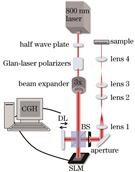
Fig. 1. Experimental setup of spatiotemporal-interference-based femtosecond laser shaping

Fig. 2. Simulation results. (a) Relative distortion fitting curve of l-q(l); (b)(c) gridded phase holograms before and after distortion correction, respectively; (d)(e) distribution of irradiance at the simulated sample when Figs. (b) and (c) are loaded on SLM

Fig. 3. Gauss Amp fitting curve for relative light intensity distribution of circular light field after the contraction

Fig. 4. Simulation results. (a)(d) Circular phase holograms before and after light-intensity correction; (b)(c) two-dimensional and one-dimensional simulated light intensity distributions when loading Fig. (a) on SLM, total power is 1.619×10^-1 W; (e)(f) two-dimensional and one-dimensional simulated light intensity distributions when loading Fig. (d) on SLM, total power is 1.352×10^-1 W

Fig. 5. Simulation result. (a)(d) Striped phase holograms before and after distortion and light-intensity correction; (b)(c) two-dimensional and one-dimensional simulated light intensity distributions when loading Fig. (a) on SLM, total power is 6.995×10^-2 W; (e)(f) two-dimensional and one-dimensional simulated light intensity distributions when loading Fig. (d) on SLM, total power is 5.073×10^-2 W; (g)(h) stainless steel surface processing images，when loading Fig. (a) or (d)

Fig. 6. Edge images of laser processing results before and after correction. (a)Before correction; (b)after correction

Fig. 7. Long stripe structure on a 500 μm thick silicon formed by stitching

Fig. 8. Simulation results. (a)(b) Two phase holograms when processing a single pixel of a QR code; (c) two-dimensional simulated light intensity distributions when loading Fig. (a) on SLM, peak irradiance is 2.077×10³ W/cm²; (d) QR code structure on stainless steel surface; (e) zoom in the view of the QR code structure

Fig. 9. Observation results. (a)LIPSS image inside QR code structure; (b)legend for measuring the LIPSS cycle

Fig. 10. Schematic of observation method for the QR code structural color

Fig. 11. Images obtained from the structure on the stainless steel surface of different α varied from large to small

Table 1.