
Yue Leng, Sheng Zhong. Thermal-Induced Drift Analysis and Algorithm Compensation Technology of Fiber Optic Gyroscope[J]. Acta Optica Sinica, 2024, 44(2): 0206003
- Acta Optica Sinica
- Vol. 44, Issue 2, 0206003 (2024)
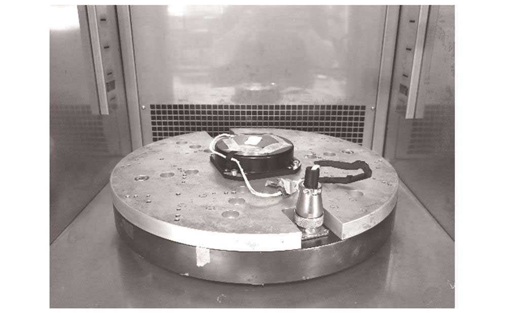
Fig. 1. Test field diagram

Fig. 2. Gyroscope output and temperature curves. (a) Zerobias curve; (b) temperature curve
Fig. 3. Temperature change process correlation curve
Fig. 4. Location diagram of two temperature sensors
Fig. 5. Output curves of two temperature sensors
Fig. 6. Process correlation considering temperature, temperature variation rate, and temperature gradient
Fig. 7. Gyroscope output contrast curves before and after compensation
Fig. 8. Process correlation curves considering coupling term factors
Fig. 9. Algorithm compensation effect considering coupling term factor
Fig. 10. Results of gyroscope experiment before algorithm compensation. (a) Temperature curve; (b) zerobias curves
Fig. 11. Results of gyroscope experiment after algorithm compensation. (a) Temperature curve; (b) zerobias curves
|
Table 1. Different compensation effects of temperature and temperature variation rate factors

Set citation alerts for the article
Please enter your email address
© Copyright 2018-2021 | Chinese Laser Press. All Rights Reserved 沪ICP备15018463号-20