• Matter and Radiation at Extremes
  • Vol. 7, Issue 5, 055902 (2022)
Jun Li1、*, Rui Yan1、2, Bin Zhao2、3, Jian Zheng2、4, Huasen Zhang5, and Xiyun Lu1
Author Affiliations
  • 1Department of Modern Mechanics, University of Science and Technology of China, Hefei 230026, China
  • 2Collaborative Innovation Center of IFSA (CICIFSA), Shanghai Jiao Tong University, Shanghai 200240, China
  • 3Department of Mathematics and Physics, Nanjing Institute of Technology, Nanjing, JiangSu 211167, China
  • 4Department of Plasma Physics and Fusion Engineering, University of Science and Technology of China, Hefei, Anhui 230026, China
  • 5Institute of Applied Physics and Computational Mathematics, Beijing 10094, China
  • show less
    DOI: 10.1063/5.0088058 Cite this Article
    Jun Li, Rui Yan, Bin Zhao, Jian Zheng, Huasen Zhang, Xiyun Lu. Mitigation of the ablative Rayleigh–Taylor instability by nonlocal electron heat transport[J]. Matter and Radiation at Extremes, 2022, 7(5): 055902 Copy Citation Text show less
    (a) Equilibrium hydrodynamic profiles of a 1.5 MJ NIF ignition target during the acceleration phase after evolving for 1 ns using the initialization of the SH model: density from the SH model (black dashed line) and from the SNB model for Kn = 0.01 (blue squares) and Kn = 0.011 (red solid line); vz from the SH model (black solid line) and from the SNB model for Kn = 0.01 (green squares) and Kn = 0.011 (orange solid line). The local Knudsen number Knloc profile (gray solid line) at t = 0 is also plotted. The three purple stars mark the locations of Knloc = {0.011, 0.010, 0.009}. (b) Linear growth rates of ARTI from the SH and SNB models for different values of Kn: the SH model for Kn = 0.01 (blue squares) and Kn = 0.011 (black triangles) and the SNB model for Kn = 0.01 (green circles) and Kn = 0.011 (red diamonds). The black triangles and blue squares are superimposed, since the SH model is local and independent of Kn. The theoretical curves are γ=(ATkg−AT2k2Va2/rd)1/2−(1+AT)kVa.20
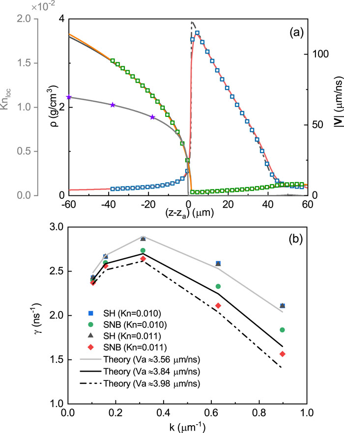
    Fig. 1. (a) Equilibrium hydrodynamic profiles of a 1.5 MJ NIF ignition target during the acceleration phase after evolving for 1 ns using the initialization of the SH model: density from the SH model (black dashed line) and from the SNB model for Kn = 0.01 (blue squares) and Kn = 0.011 (red solid line); vz from the SH model (black solid line) and from the SNB model for Kn = 0.01 (green squares) and Kn = 0.011 (orange solid line). The local Knudsen number Knloc profile (gray solid line) at t = 0 is also plotted. The three purple stars mark the locations of Knloc = {0.011, 0.010, 0.009}. (b) Linear growth rates of ARTI from the SH and SNB models for different values of Kn: the SH model for Kn = 0.01 (blue squares) and Kn = 0.011 (black triangles) and the SNB model for Kn = 0.01 (green circles) and Kn = 0.011 (red diamonds). The black triangles and blue squares are superimposed, since the SH model is local and independent of Kn. The theoretical curves are γ=(ATkgAT2k2Va2/rd)1/2(1+AT)kVa.20
    (a) Bubble and spike trajectories from the SH and SNB models vs Zt in the λ = 7 µm, Kn = 0.01 cases, where Zt≡∫0t∫0t′′g(t′)dt′dt′′ is the displacement function commonly used in theoretical descriptions of time-dependent acceleration histories. (b) Ratio of bubble velocities to classical values. The symbols represent the simulations and the curves are from the analytical model given by Eq. (8). (c) Average vorticity inside the bubble volume within a length 1/k below the bubble vertex, as illustrated in Fig. 3(a).
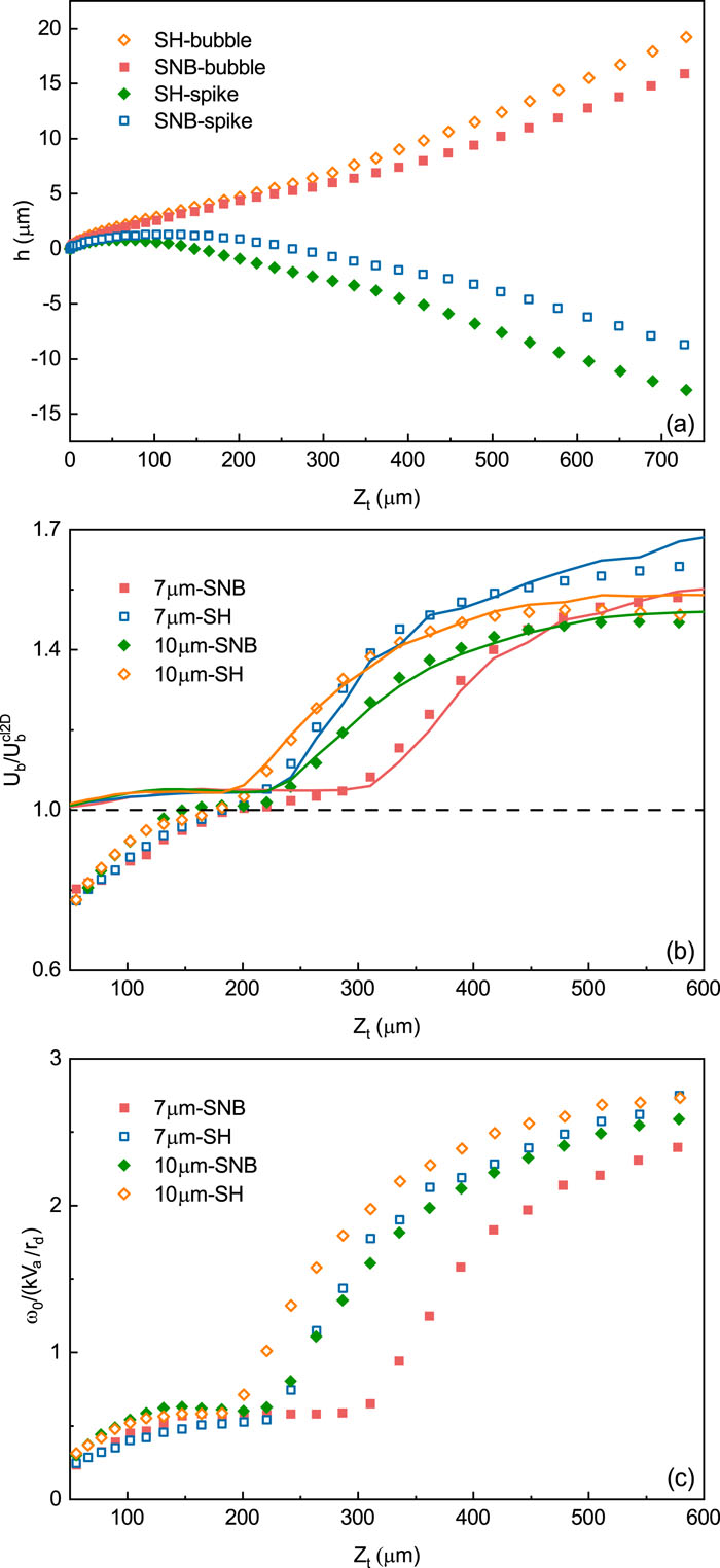
    Fig. 2. (a) Bubble and spike trajectories from the SH and SNB models vs Zt in the λ = 7 µm, Kn = 0.01 cases, where Zt0t0tg(t)dtdt is the displacement function commonly used in theoretical descriptions of time-dependent acceleration histories. (b) Ratio of bubble velocities to classical values. The symbols represent the simulations and the curves are from the analytical model given by Eq. (8). (c) Average vorticity inside the bubble volume within a length 1/k below the bubble vertex, as illustrated in Fig. 3(a).
    Simulation results for the 10 μm-SNB case at t = 1.7 ns (Zt = 180 µm). (a) Density. The volume marked inside the bubble is within 1/k below the bubble tip. (b) Temperature contour with heat flux vectors. (c) Vorticity. (d) Baroclinic source ω̇baro≡−∇P×∇ρ/ρ2. (e) Zoomed-in image of the vorticity and baroclinic source near the RTI interface. The hydrodynamic contours in the SH case are qualitatively similar to those in the SNB case.
    Fig. 3. Simulation results for the 10 μm-SNB case at t = 1.7 ns (Zt = 180 µm). (a) Density. The volume marked inside the bubble is within 1/k below the bubble tip. (b) Temperature contour with heat flux vectors. (c) Vorticity. (d) Baroclinic source ω̇baroP×ρ/ρ2. (e) Zoomed-in image of the vorticity and baroclinic source near the RTI interface. The hydrodynamic contours in the SH case are qualitatively similar to those in the SNB case.
    (a) Density profile and the heat flux correction term QSNB − QSH along the spike axis at t = 2.1 ns (Zt = 286 µm) in the 7 µm SNB case. The density profile of the SH case at the same time is plotted as the dash-dotted line for comparison. QSNB and QSH are calculated using the density and temperature profiles from the SNB model. (b) Dependence of the volume-averaged baroclinic source −∇P × ∇ρ/ρ2 on the dimensionless quantity kLspike for both SH and SNB simulations.
    Fig. 4. (a) Density profile and the heat flux correction term QSNBQSH along the spike axis at t = 2.1 ns (Zt = 286 µm) in the 7 µm SNB case. The density profile of the SH case at the same time is plotted as the dash-dotted line for comparison. QSNB and QSH are calculated using the density and temperature profiles from the SNB model. (b) Dependence of the volume-averaged baroclinic source −∇P × ∇ρ/ρ2 on the dimensionless quantity kLspike for both SH and SNB simulations.
    Jun Li, Rui Yan, Bin Zhao, Jian Zheng, Huasen Zhang, Xiyun Lu. Mitigation of the ablative Rayleigh–Taylor instability by nonlocal electron heat transport[J]. Matter and Radiation at Extremes, 2022, 7(5): 055902
    Download Citation