Fig. 1. Schematic illustration of the research model and the obtained inflection point. (a) 3D schematic diagram of a dielectric microcylinder illuminated by an incident plane EM wave. (b) 2D representation of the research model in (a). Green solid lines show the process of a plane wave propagation through the microcylinder. RSC, region of slow change; RRC, region of rapid change; RWC, region of weak contribution; O, origin of coordinates; r, radius of microcylinder; nm, ne, refractive indices of microcylinder and environmental medium; θiem, θime, angles of incidence; θrem, θrme, angles of refraction; Sie, Sm, Soe, slopes of the transmission rays. (c) Ray trajectories of the plane light wave transmission through RWC (light-gray solid line), RRC (magenta-pink solid line), and RSC (cyan-blue solid line). Inset: 12× enlarged view of the selected area in RWC. (d) Slope of emergent ray (Soe) and position of emitting point along the x axis (Lx) as a function of the incidence angle (θiem). θiem±, angle of incidence corresponding to the jump point between positive and negative values of the slope curve; θiemRW, angle of incidence corresponding to the dividing point between RWC and RRC. (e) Natural log of the slope function ln(Soe) with respect to the initial incidence angles θiem. (f) Second derivative values of the slope curve shown in (e). Inset: enlarged view of d2[ln(Soe)]/dθiem2 in the range of θiem∈(−55.08°,−35.08°).

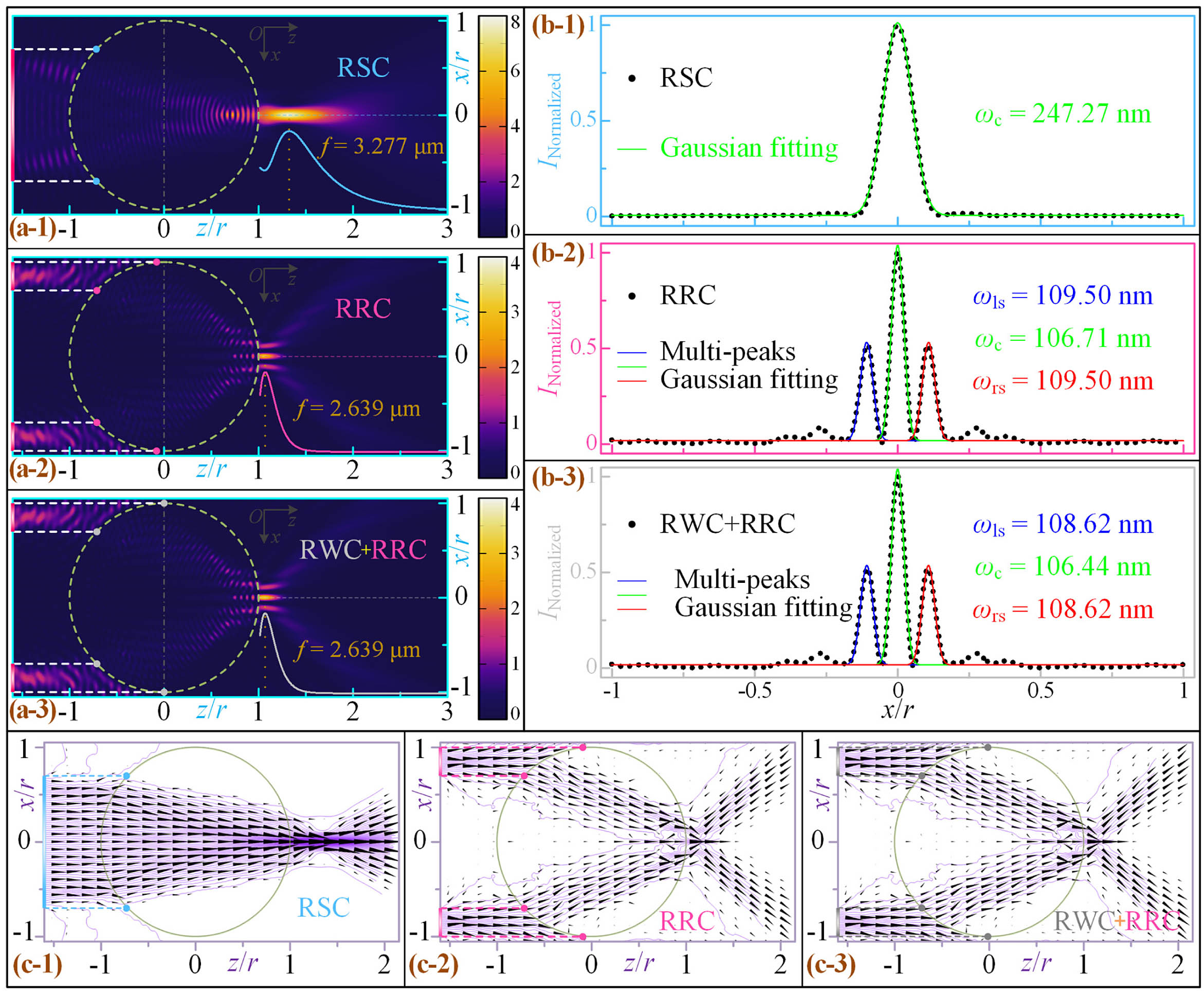
Fig. 2. 2D optical field distributions of light illuminating the (a-1) RSC, (a-2) RRC, and (a-3) composite region of “RWC + RRC” obtained from FEM-based full-wave simulations. The model parameters are: λ0=400  nm, r=2.5  μm, nm=1.5, ne=1.0. Insets: normalized spatial intensities of the focused light field from x/r=0, z/r=1 to x/r=0, z/r=3 for the cases of RSC (cyan-blue solid line), RRC (magenta-pink solid line), and “RWC + RRC” (light-gray solid line) irradiated by the plane wave. The vertical dotted line indicates the position of the focal point and focal distance f for each figure. (b-1)–(b-3) Normalized transverse light field profiles (black dots) at the focal point along x direction and the single-peak, multi-peak Gaussian fitting curves corresponding to (a-1)–(a-3), respectively. (c-1)–(c-3) Poynting vector distributions (black conical arrows) and energy flow streamlines (purple solid curves) for the cases of irradiation areas located in the regions of RSC, RRC, and “RWC + RRC,” respectively.

Fig. 3. Inflection point between RSC and RRC of the first LRI for the model of plane-wave-illuminated microcylinder varies with the RIC of microcylinder and environment medium. (b) Position distributions of the emitting points L relative to the incidence angles θiem along x direction for the cases of RIC=1.60, RIC=2, and RIC=1.35. Insets: schematic illustrations of the ray-tracing process of propagation light beam and trajectories of the emitting points for RIC=1.60, RIC=2, and RIC=1.35. A, incident point; L, emitting point.

Fig. 4. (a) Working distance Wd and (b) transverse beam width (central main lobe) ωc of light focusing as a function of RIC and incidence angle at the inflection point associated with RIC for the cases of RSC and C-RRC illuminated by the plane wave. (c) Slope curves of emergent rays Soe and (d) corresponding position distributions of emitting points Lx as a function of Ax/r (ratio of the x coordinate of incident points Ax to the radius of the microcylinder) for different RICs. The magenta-pink and cyan-blue coordinate axes in (c) and the magenta-pink and cyan-blue shadow areas in (d) are relevant to the illumination regions of RRC and RSC, respectively.

Fig. 5. Schematic diagrams illustrate the existence of (a-1) PNJ and (a-2) PH for the cases of |E|=|Eu|=|El| and |E|=|Eu|, |El|≠|Eu|, respectively. |Eu|, |Em|, and |El| correspond to the electric field intensity of light irradiated to the C-RRC above, RSC, and C-RRC below, respectively. |E| is the independent variable set. λu, λm, and λl are the wavelengths of the plane waves illuminating each area, where λu=λl=λm=λ0=400  nm. (b) Modulation of PNJ key parameters (working distance Wd and transverse beam width ωc) by varying |E|/|Em| from zero to ∞ for the case of |E|=|Eu|=|El|. Four intervals of [0.1, 0.5], [1, 5], [10, 50], [100, 500] with respective step sizes of 0.05, 0.5, 5, and 50 are contained within the range of the independent variables. ARC, average rate of change, stands for dividing the difference of Wd by the difference of |E|/|Em| for the two endpoints in each interval. Insets: five examples of light field distributions in terms of contour lines. The gray dots mark the location of the Imax.

Fig. 6. PHs formed at the rear surface of the microcylinder under illumination conditions of (a) |Eu|/|Em|=0, |Em|=1, |El|/|Em|=1.5 and (b) |Eu|/|Em|=3.5, |Em|=1, |El|/|Em|=0.5. (c) Optical field distribution of the trajectories marked with Cambridge-blue and wine-red dotted curves in (a) and (b). (d) Transverse optical field profiles at the focal point along x direction corresponding to the cases of |Eu|/|Em|=0, |El|/|Em|=1.5 (Cambridge-blue curve), and |Eu|/|Em|=3.5, |El|/|Em|=0.5 (wine-red curve).

Fig. 7. Modulation of PH key parameters (Wd and ωc) by varying |Eu|/|Em| from zero to five in the cases of |El|/|Em|=0 and |El|/|Em|=0.3. The light-red and olive dotted lines marked in the figure indicate the vertical positions of evanescent decay length (1/2π) and diffraction limit (λ0/2).

Fig. 8. Bending angles (δb) with respect to |Eu|/|Em| from zero to five in the cases of |El|/|Em|=0 and |El|/|Em|=0.3. Insets: electric field distributions and bending angles for the cases of |El|/|Em|=0, |Eu|/|Em|=1.25 and |El|/|Em|=0.3, |Eu|/|Em|=2.25. Five-pointed stars marked with dotted circle: PNJ generated at |Eu|=|El|.

Fig. 9. Distributions of energy flow streamlines of (a-1) RRC and (a-2) “RWC + RRC” on the first LRI illuminated by a plane wave. From the central symmetry axis of the microcylinder to both sides, the 11 streamlines are represented by Arabic numbers 1–11 and marked with small circles. (b) Relative differences in x positions of the 11 streamlines for the two cases. The effective widths are the distance between two points of intensity I equaling Imax/e2 for the central lobe, and between two points of I=Ils-max/e2 on the left and I=Irs-max/e2 on the right for the left and right sidelobes, respectively.

Fig. 10. Contour plots of optical field distributions for the illumination conditions of (a) |Em|=1, |El|/|Em|=0, |Eu|/|Em|=2.5; (b) |Em|=1, |El|/|Em|=0, |Eu|/|Em|=2.75; (c) |Em|=1, |El|/|Em|=0, |Eu|/|Em|=3; and (d) |Em|=1, |El|/|Em|=0, |Eu|/|Em|=3.25. Imax, maximum light intensity in the entire optical field distribution; Il, local maximum light intensity within the selected area. The large circles drawn with solid black lines denote a closed interval containing Imax point and closed contour curve. The small circles drawn with solid black lines and dotted black lines denote the closed interval containing Il point and closed contour curve and the unclosed intervals containing only Il point. The x coordinate and z coordinate variables are in micrometers.

Fig. 11. (a) Schematic diagram used to define the bending angle of PH. “B,” selected arc line on the boundary between the microcylinder and environmental medium; Ibmax, maximum value of the light intensity distribution curve of arc line “B”; “R,” selected rectangular area containing part of the contour curve with light intensity of Imax/e2. The marked green, red, and blue dots are, respectively, the start point, Imax point, and end point. The angle between two pink lines is the bending angle δb. (b) Optical field distribution of an example with |Eu|/|Em|/|El|=1.75:1:0.3. The radius of the microcylinder is r=2.5  μm. The refractive indices of the microcylinder and environmental medium are nm=1.5 and ne=1.0, respectively. The wavelength of the incident plane wave is λu=λl=λm=λ0=400  nm. Light intensity distributions in (c) arc line “B” and (d) Imax/e2 contour curve within rectangular area “R.” The highlighted sphere in (c) and circle in (d) are the start point (Ibmax) and end point, respectively.

Fig. 12. Schematic diagram of a plane-wave-illuminated microcylinder made of composite materials. The refractive indices of the upper, middle, and lower parts of the microcylinder are nu, nm, and nl, respectively. The radius of the microcylinder is r. (b) Optical field distribution of the PH formed by composite microcylinder at nu=nm=1.5, nl=1.8, r=2.5  μm, and λ0=400  nm. (c) Enlarged view of the selected area in (b). The yellow circles and the arguments I, II, III, IV, and V marked in the figure point out five deflection points. The blue curve represents a contour line with intensity of Imax/e2.