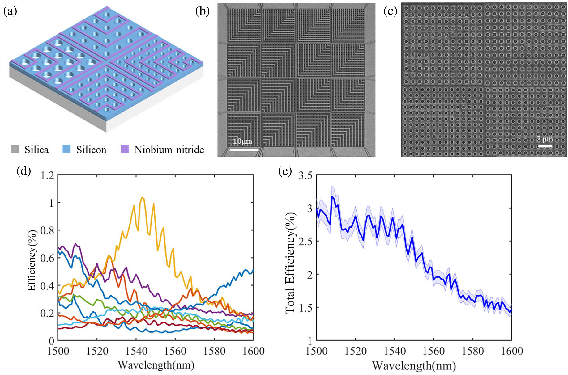
Fig. 1. Sketch of the proposed photon counting reconstructive spectrometer and SEM pictures of the prototype device. (a) Sketch of the spectrometer, which is a metasurface array with SNSPDs in different regions. (b) SEM picture of the full view of the device. (c) SEM picture of four spectral sensing units in the device. (d) Spectral responses of all spectral sensing units. (e) Spectrum of total detection efficiency of this device. The shaded region represents the uncertainty of detection efficiency at each wavelength.

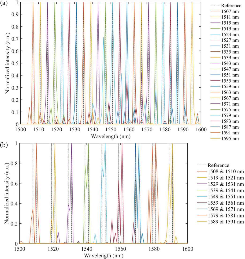
Fig. 2. Spectrometer characterizations from 1500 nm to 1600 nm. (a) Reconstruction results of attenuated monochromatic lights at different wavelengths. (b) Reconstruction results of two monochromatic lights with a wavelength interval of 2 nm at different wavelength settings.

Fig. 3. Statistics of the RMSE of the reconstructed spectrum for a specific broadband light under different measurement time T. The upper x axis is the average photon counts recorded by the device, which are calculated by T and the total photon count rate. Error bar is the standard deviation of the RMSE. Inset images are typical reconstruction results under RMSEs of 0.23, 0.15, 0.10, and 0.05.

Fig. 4. (a) Schematic diagram of the experimental setup of the spectral response calibration. (b) Photon count rates of the device in 1 h.

Fig. 5. Spectral responses of different detection units under two different polarizations. Blue and orange lines show the results under two different input polarization states, under which the device achieves its maximum and minimum detection efficiencies at 1550 nm, respectively.

Fig. 6. Spectral responses of SNSPDs in the sample without metasurfaces. (a) SEM picture of the sample. (b) Spectral responses of the SNSPDs. (c) Total efficiency of the sample.

Fig. 7. Spectrometer characterizations from 1350 nm to 1629 nm. (a) Spectral responses of each spectral sensing unit. (b) Total detection efficiency spectrum of the device. The shaded region represents the uncertainty of detection efficiency at each wavelength. (c) Reconstruction results of attenuated monochromatic lights at different wavelengths. (d) Typical reconstruction result of an attenuated broadband light provided by an EDF ASE source. (e)–(h) Reconstruction results of two monochromatic lights near 1550 nm with wavelength intervals of 6 nm, 9 nm, 12 nm, and 15 nm, respectively.

Fig. 8. Experiment results of fast spectral measurement. (a) Schematic sketch of the temporal wavelength variation of the attenuated monochromatic light. (b)–(d) Reconstructed spectra measured under different settings of Tw and δTw when the wavelength of the attenuated monochromatic light sweeps from 1547 nm to 1554 nm. (b) Tw=1 s and δTw=100  ms; (c) Tw=0.5  s and δTw=50  ms; (d) Tw=0.2  s and δTw=20  ms.