
Bo Song, Wei Fang, Lili Du, Wenyu Cui, Tao Wang, Weining Yi. Simulation method of high resolution satellite imaging for sea surface target[J]. Infrared and Laser Engineering, 2021, 50(12): 20210127
- Infrared and Laser Engineering
- Vol. 50, Issue 12, 20210127 (2021)
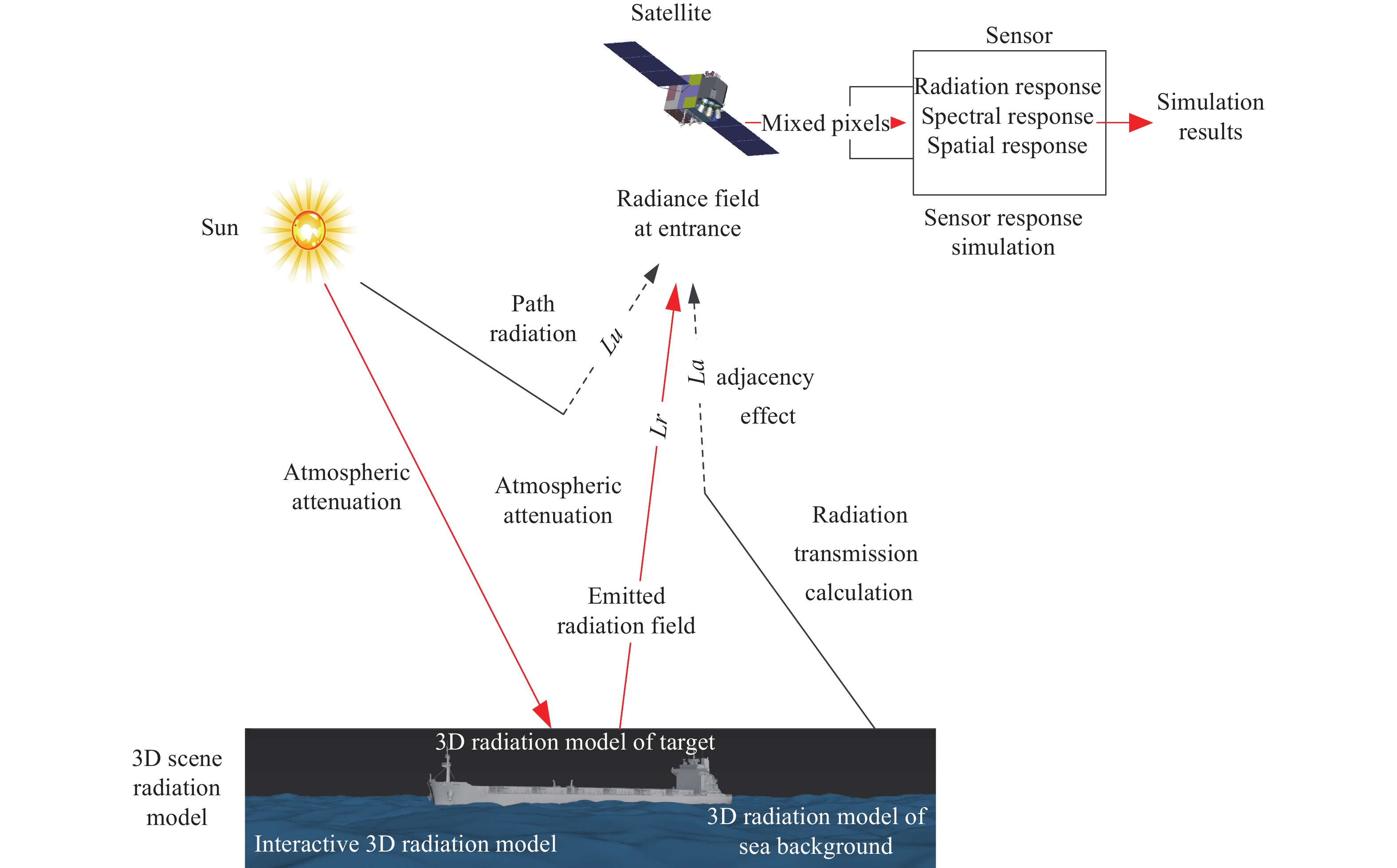
Fig. 1. General flow chart of satellite imaging simulation
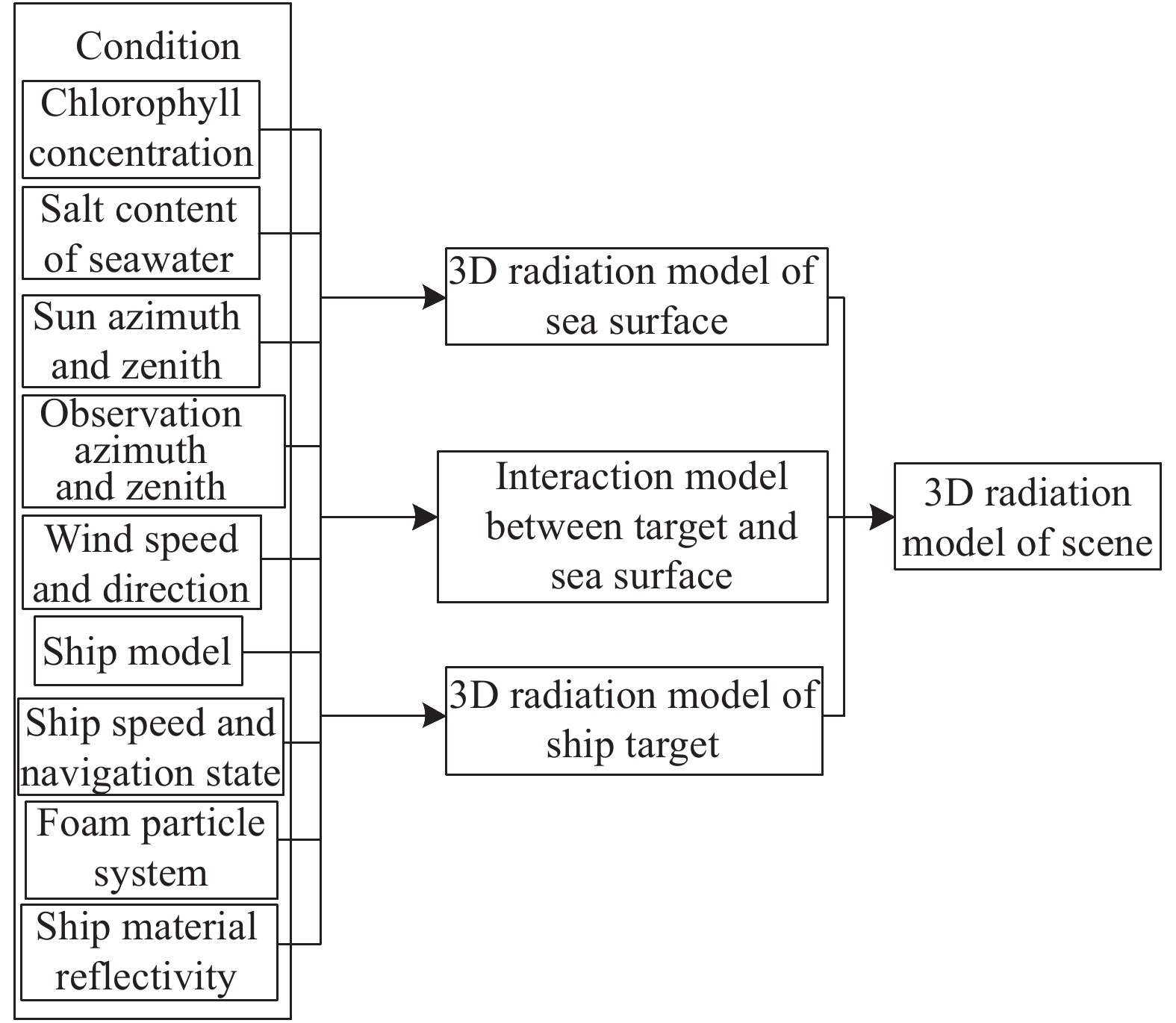
Fig. 2. Construction of 3D radiation model of sea scene
Fig. 3. Schematic diagram of sea background modeling
Fig. 4. 3D structure of sea surface under different wind speeds
Fig. 5. Directional reflectance of seawater without foam covering area calculated by OCEABRDF model
Fig. 6. Reflectivity spectrum of sea surface foam
Fig. 7. Modeling sketch of sea surface target
Fig. 8. 3D model of cargo ship
Fig. 9. Reflectivity information of hull part
Fig. 10. Sketch of coupling modeling between target and sea background
Fig. 11. Schematic diagram of scene 3D radiation model
Fig. 12. Schematic diagram of ray tracing simulation of multiple reflections of radiant energy inside the scene
Fig. 13. Simulation zero line of sight radiation distribution under turning state
Fig. 14. Simulated atmospheric PSF under different visibility
Fig. 15. Spectral response function of GF6 PMS in Pan band
Fig. 16. Satellite edge map (a) and calculated camera point spread function (b) and MTF curve (c)
Fig. 17. Simulation results under different conditions. (a) Different ship targets; (b) Different sailing speed of the same ship; (c) Observation results of different resolutions; (d) Observation results of different atmospheric conditions
Fig. 18. Satellite measurement results and simulation results
Fig. 19. Pseudo color map of satellite measurement results and simulation results
Fig. 20. Comparison of gray histogram between satellite measured results and simulation results
|
Table 1. OCEABRDF input parameter table
|
Table 2. Cargo ship model information
|
Table 3. Simulation conditions
| ||||||||||||||||||||||||||||||||||||||||||||||
Table 4. Comparison of simulation results and measured results

Set citation alerts for the article
Please enter your email address
© Copyright 2018-2021 | Chinese Laser Press. All Rights Reserved 沪ICP备15018463号-20