Aberration correction for multiphoton microscopy using covariance matrix adaptation evolution strategy

Ke Wang; Lei Zheng; Mengyuan Qin; Wanjian Zhang; Xiangquan Deng; Shen Tong; Hui Cheng; Jie Huang; Jincheng Zhong; Yingxian Zhang; Ping Qiu

doi:10.3788/COL202321.051701

Abstract

Multiphoton microscopy is the enabling tool for biomedical research, but the aberrations of biological tissues have limited its imaging performance. Adaptive optics (AO) has been developed to partially overcome aberration to restore imaging performance. For indirect AO, algorithm is the key to its successful implementation. Here, based on the fact that indirect AO has an analogy to the black-box optimization problem, we successfully apply the covariance matrix adaptation evolution strategy (CMA-ES) used in the latter, to indirect AO in multiphoton microscopy (MPM). Compared with the traditional genetic algorithm (GA), our algorithm has a greater improvement in convergence speed and convergence accuracy, which provides the possibility of realizing real-time dynamic aberration correction for deep in vivo biological tissues.

Keywords

1700-nm window adaptive optics covariance matrix adaptation evolution strategy multiphoton microscopy

1. Introduction

In recent years, multiphoton microscopy (MPM) has made great progress in imaging biological tissues, especially brain tissue, due to its advantages of noninvasiveness and deep-tissue penetration^[1–5]. Among the various MPM modalities using different excitation wavelengths, 3-photon microscopy (3PM) excited at the 1700-nm window is intriguing in that it enables the largest brain imaging depth in vivo so far^[5]. However, optical aberration arising from the brain tissue distorts the focus, which further limits maximum imaging depth.

In order to overcome the optical aberration, adaptive optics (AO) has been introduced into MPM^[6–8]. There are two types of AO, one of which requires direct wavefront detection with a wavefront sensor (direct AO), while the other type does not require a wavefront sensor and calculates the wavefront by iterative algorithms (indirect AO). Compared with direct AO, indirect AO is easier and cheaper to implement. However, indirect AO requires algorithmic iterations to calculate the wavefront and compensate accordingly, since no wavefront sensor is required, and it therefore requires much more time and cost than direct AO. Many algorithms have been developed for indirect AO, such as the hill climbing algorithm^[9], the genetic algorithm (GA)^[10], the particle swarm algorithm (PSO)^[11], and the simulated annealing algorithm (SA)^[12]. These algorithms significantly accelerate the process of indirect AO, but the speed of optimization is still not high enough to deal with high dynamic media like in vivo biological tissue. In addition, these algorithms involve stochastic variables in the optimization and are sensitive to the initial condition and local optimum^[13], which may affect the resultant aberration correction. Therefore, it is desirable to develop a new optimization method with a high speed and strong capability of global search.

We have found that indirect AO optimization is quite similar to the black-box optimization problem^[14], so we expect that the algorithm applicable to black-box optimization can be directly applied to indirect AO. Here, we propose a new approach to indirect AO based on an algorithm called covariance matrix adaptation evolution strategy (CMA-ES)^[15]. The CMA-ES is a widely used algorithm for black-box optimization problems and has proved to be very effective^[16]. Through both numerical simulation and experiment, we show that the CMA-ES has a faster convergence speed and higher accuracy than the GA in indirect AO, which provides a new approach for fast in vivo aberration correction and provides the possibility of further improving the maximum multi-photon imaging depth.

Sign up for Chinese Optics Letters TOC. Get the latest issue of Chinese Optics Letters delivered right to you！Sign up now

2. Methods

2.1. Basic principle of CMA-ES

The CMA-ES is an evolutionary algorithm based on Gaussian mutation and deterministic selection. Evolutionary strategies are stochastic search methods inspired by the principles of biological evolution typically using a multivariate normal mutation distribution. The CMA-ES is considered to be one of the best choices against ill-conditioned, non-convex black-box optimization problems in the continuous domain^[16]. The core idea of the CMA-ES is to deal with the dependence between variables and scaling by adjusting the covariance matrix in the normal distribution^[15]. The solution of the algorithm is updated by $x_{k}^{(g + 1)} \sim m^{(g)} + σ^{(g)} N (0, C^{(g)}), k = 1, \dots, λ .$ (1)

$x_{k}^{(g + 1)}$ denotes the $k$ th solution of the $(g + 1)$ th generation, the symbol $\sim$ represents that the left and right parts of the symbol are subject to the same distribution, and $m^{(g)}$ denotes the mean value of the $g$ th generation search distribution, which can be updated by $m^{(g + 1)} = m^{(g)} + c_{m} \sum_{i = 1}^{µ} w_{i} (x_{i : λ}^{(g + 1)} - m^{(g)}),$ (2)where $c_{m} \leq 1$ denotes the learning rate of $m$ , $µ \leq λ$ denotes the size of the parent sample, and $\sum_{i = 1}^{µ} w_{i} = 1,$ (3)where $w_{i} (1 \leq i \leq µ)$ denotes the weights of sample selection, and $σ^{(g)}$ denotes the step length of the $g$ th generation, which can be updated by $σ^{(g + 1)} = σ^{(g)} \exp (\frac{c_{σ}}{d_{σ}} (\frac{‖ p_{σ}^{(g + 1)} ‖}{E ‖ N (0, I) ‖} - 1)),$ (4)where $p_{σ}^{(g + 1)} = (1 - c_{σ}) p_{σ}^{(g)} + \sqrt{c_{σ} (2 - c_{σ}) \frac{1}{\sum_{i = 1}^{µ} w_{i}^{2}} C^{(g)}} - \frac{1}{2} \frac{m^{(g + 1)} - m^{(g)}}{σ^{(g)}}$ (5)denotes the conjugate evolutionary path, $c_{σ} \leq 1$ denotes the learning rate of $σ$ , $d_{σ}$ is a constant approximately equal to 1, and $C^{(g)}$ denotes the covariance matrix of the $g$ th generation. It can be updated by $C^{(g + 1)} = (1 - c_{µ}) C^{(g)} + c_{µ} \frac{1}{{(σ^{(g)})}^{2}} \sum_{i = 1}^{µ} w_{i} (x_{i : λ}^{(g + 1)} - m^{(g)}) {(x_{i : λ}^{(g + 1)} - m^{(g)})}^{⊤},$ (6)where $c_{µ} \leq 1$ denotes the learning rate of $µ$ .

Similar to the GA, the dimensionality of the solution, the size of the population, and the maximum number of iterations need to be determined before starting the CMA-ES. Then, given the initial search point and initialized parameters ( $C^{(0)} = I$ and $p^{(0)} = 0$ ), the iterative computation is carried out and stops after the maximum number of iterations is reached, and the result is outputted.

2.2. Experimental setup

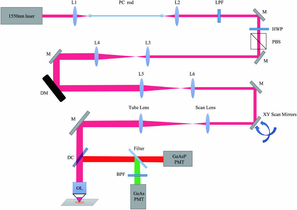
Our experimental setup (Fig. 1) is similar to that used in Ref. [4]. The 1680-nm soliton source was generated through the soliton self-frequency shift, pumped by a 500-fs, 1550-nm femtosecond laser (FLCPA-02CSZU, Calmar) at 1 MHz. A 44-cm photonic crystal (PC) rod (SC-1500/100-Si-ROD, NKT Photonics) was used to shift the soliton to 1680 nm. An f = 100 mm C-coated achromatic lens (AC254-100-C-ML, Thorlabs) and an f = 75 mm C-coated achromatic lens (AC254-75-C-ML, Thorlabs) were used to focus the pump laser into the PC rod and to collimate the output solitons, respectively. The residual pump was removed by a 1650-nm long-pass filter (customized 1650lpf, Mei Zhou Yi Zhao Photonics Technology). The filtered solitons were expanded by an f = 35 mm lens (AC254-35-C-ML, Thorlabs) and an f = 150 mm lens (AC254-150-C-ML, Thorlabs) to fill all the apertures of the deformable mirror (DM97-15, Alpao). The solitons reflected by the deformable mirror were condensed by an f = 500 mm lens (AC254-500-C-ML, Thorlabs) and an f = 150 mm lens (AC254-150-C-ML, Thorlabs), and then entered into the dual-axis galvo mirror systems (GVS002, Thorlabs). After that the solitons were expanded by an f = 50 mm scan lens (AC254-50-C-ML, Thorlabs) and an f = 200 mm tube lens (AC508-200-C-ML, Thorlabs). A water immersion objective lens (XLPLN25XWMP2, NA = 1.05, Olympus) with 2-mm working distance (WD) was used.

Figure 1.Experimental setup. L1, f = 100 mm lens; L2, f = 75 mm lens; LPF, 1650-nm long-pass filter; HWP, half-wave plate; PBS, polarization beam splitter cube; L3, f = 35 mm lens; L4, f = 150 mm lens; L5, f = 500 mm lens; L6, f = 150 mm lens; DC, dichroic mirror; OL, objective lens; BPF, bandpass filter.

A GaAsP photomultiplier tube (PMT, PMT2102, Thorlabs) with a 525/70-nm bandpass filter (ET525/70M-2p, Chroma) was used to detect third harmonic generation (THG) signals from the brain slice, and 3PF images of fluorescent beads were acquired using a GaAsP PMT (H7422p-40, Hamamatsu) with a 630/92-nm bandpass filter (FF01-630/92-25, Semrock). Image acquisition and processing were performed using ScanImage (Vidrio Technology, Ashburn, Virginia) and ImageJ (NIH, Bethesda, Maryland), respectively. During the iteration of the adaptive algorithm, the acquisition speed was 0.49 ms/line with a resultant frame rate of 16 frames/s for a pixel size of $128 \times 128$ . For tissue imaging, the acquisition speed was 2 ms/line with 2 averages, with a resultant frame rate of 0.5 frame/s for a pixel size of $512 \times 512$ .

2.3. Sample preparation

The fluorescent bead sample was prepared using 1 µm fluorescent beads (F13083, ThermoFisher) mixed with a 1.5% agarose solution at a ratio of 1:500. The mice (Balb/c) were all from the Guangdong Medical Laboratory Animal Center, between ages six and eight weeks. The brain was removed after isoflurane euthanasia and decapitation of the mouse. Then, it was rinsed with saline. Coronal cortical slices of 350 µm thick were cut in a Vibratome (ZQP-86, Shanghai Zhixin Instrument Co., Ltd.) at 4°C in artificial cerebrospinal fluid (ACSF, PH 7.3, CZ0524, Leagene). Animal procedures were reviewed and approved by Shenzhen University.

3. Results and Discussion

3.1. Performance verification by numerical simulation

To verify the performance of indirect AO based on CMA-ES, we first carried out a numerical simulation. Due to the correlation between Zernike polynomials and aberrations^[17], we chose to model the wavefront aberration using the first 30 orders Zernike polynomials, with the polynomial coefficients generated randomly and subject to normal distribution. Next, we used the coefficients of the Zernike polynomials as variables and the root mean square (RMS) value of the optimized wavefront as feedback for iterative optimization with the GA and the CMA-ES, respectively. The overall process is shown in Fig. 2. The population size of both algorithms was 20, and the maximum number of iterations was 100, where the crossover rate and mutation rate of the GA were 0.8 and 0.2, respectively, and the σ of the CMA-ES was $π / 10$ .

Figure 2.Simulation process schematic. (a) The GA process schematic, and (b) the CMA-ES process schematic.

As shown in Fig. 3(a), the initial wavefront RMS value is 5.4821 µm, and the wavefront RMS value is reduced to 1.4700 µm after the GA optimization. After the CMA-ES optimization, the wavefront RMS value is reduced to 0.0628 µm, which is nearly 20 times lower than the RMS value of the wavefront optimized by the GA. This indicates that the initial distortion wavefront is closer to the ideal plane wavefront after the CMA-ES optimization than after the GA optimization, and the iteration curve in Fig. 3(b) also shows that the CMA-ES has faster convergence speed and higher accuracy than the GA. As can be seen from the iteration curve, the wavefront RMS value has been optimized to about 1.5 µm after 30 iterations of the CMA-ES, while the GA takes a full 100 iterations to achieve nearly the same result.

Figure 3.Comparison of the GA and the CMA-ES by numerical simulation. (a) The original aberrated wavefront (left), the wavefront corrected by GA (middle), and the wavefront corrected by CMA-ES (right). (b) The iteration curve comparison.

3.2. System aberration correction

Next, we performed a system aberration correction due to the microscope. We select the first 30 Zernike polynomial coefficients (except for the tip, tilt) as variables for optimization. The approach taken is similar to the simulation experiment, except that the objective function value is changed from the wavefront RMS to the fluorescence intensity. The results are shown in Fig. 4. In the 3PF image of a fluorescent bead [Fig. 4(a)], we can see that after correction by the GA, the fluorescence intensity of the bead has been enhanced, so the axial resolution is improved. After correction by the CMA-ES, the fluorescence intensity is further enhanced compared to that after the GA correction. This improvement in fluorescence intensity is due to the improvement on axial resolution. We measured the full-width at half-maximum (FWHM) of the fluorescence on the $z$ -axis and calculated the point spread function (PSF) of the $z$ -axis from the following equation: ${PSF}_{z} = \sqrt{{FWHM}^{2} - R^{2}},$ (7)where $R$ denotes the diameter of fluorescent beads. The FWHM without correction, the FWHM after the GA correction, and the FWHM after the CMA-ES correction are 4.17 µm, 4.00 µm, and 3.66 µm, respectively. Therefore, the calculated $z$ -axis PSFs are 4.05 µm, 3.87 µm, and 3.52 µm, respectively. The calculated results show that the CMA-ES based aberration correction method has improved the $z$ -axis resolution of the MPM. In the iteration curve in Fig. 4(c), it can be seen that both the CMA-ES and the GA complete convergence at 20 iterations. Both the CMA-ES and the GA converge at 20 iterations. However, the CMA-ES converges to a more optimal solution compared to the GA, which means that the CMA-ES has higher convergence accuracy in this case. The results above are in agreement with our numerical simulation, further verifying the effectiveness of the method.

Figure 4.System aberration correction results. (a) The comparison of the fluorescent bead before and after corrections (left, without correction; middle, correction by GA; right, correction by CMA-ES). (b) The axial resolution comparison. (c) The iteration curve comparison.

3.3. Brain slice aberration correction

It is well known that the aberrations in biological tissues are more complex than those in a microscope^[18]. To further test our approach, we performed aberration correction on the brain slice during THG imaging. We first acquired uncorrected THG images of brain slices and then acquired THG images after the GA and the CMA-ES optimization. The entire imaging process is similar to Ref. [8]. The optimization method is the same as the system aberration correction method. As the results shown in Fig. 5(a), we can see that after correction by both the GA and the CMA-ES, both the image resolution and the THG signal are obviously improved. As a quantitative comparison, Fig. 5(b) shows the line profiles of THG signals plotted along the lines at the same imaging position in Fig. 5(a). After the GA correction of the underlined part, the THG signal is improved by 60%, and after the CMA-ES correction, the THG signal is improved by 95%. This can also be seen in the iteration curve in Fig. 5(c). The GA converges to a local optimum after about 15 iterations, while the CMA-ES can converge to a more optimal solution. This shows that even in the case of complex aberrations introduced by biological tissue, the CMA-ES still performs better than the GA.

Figure 5.Brain slice aberration correction result. (a) The Brain slice THG image (left, without correction; middle, correction by GA; right, correction by CMA-ES). (b) The line profile of the underlined THG signal in (a). (c) The comparison of the iteration curves.

4. Conclusion

In MPM, indirect AO has become a versatile method to overcome the aberrations caused by deep tissue^[18]. Different algorithms have been developed for indirect AO, and efforts toward this target have constantly been made. Here, we proposed and demonstrated the application of a new algorithm, the CMA-ES, for indirect AO and compare its performance to another popular algorithm, the GA. Both our numerical simulation and experimental results show that the CMA-ES has faster convergence speed and higher convergence accuracy than the GA in terms of aberration correction, which has potential in fast biological tissue aberration correction. Our technology also shows an analogy between the black-box optimization problem and indirect AO, which means algorithms commonly used for black-box optimization can be applied to indirect AO. In the future, we may apply this technology to in vivo imaging.

References

[1] W. Denk, J. H. Strickler, W. W. Webb. Two-photon laser scanning fluorescence microscopy. Science, 248, 73(1990).

[2] L.-C. Cheng, N. G. Horton, K. Wang, S. J. Chen, C. Xu. Measurements of multiphoton action cross sections for multiphoton microscopy. Biomed. Opt. Express, 5, 3427(2014).

[3] N. G. Horton, K. Wang, D. Kobat, C. G. Clark, F. W. Wise, C. B. Schaffer, C. Xu. In vivo three-photon microscopy of subcortical structures within an intact mouse brain. Nat. Photonics, 7, 205(2013).

[4] H. Liu, X. Chen, X. Deng, Z. Zhuang, S. Tong, W. Xie, J. Li, P. Qiu, K. Wang. In vivo deep-brain blood flow speed measurement through third-harmonic generation imaging excited at the 1700-nm window. Biomed. Opt. Express, 11, 2738(2020).

[5] H. Liu, X. Deng, S. Tong, C. He, H. Cheng, Z. Zhuang, M. Gan, J. Li, W. Xie, P. Qiu, K. Wang. In vivo deep-brain structural and hemodynamic multiphoton microscopy enabled by quantum dots. Nano Lett., 19, 5260(2019).

[6] D. Sinefeld, H. P. Paudel, D. G. Ouzounov, T. G. Bifano, C. Xu. Adaptive optics in multiphoton microscopy: comparison of two, three and four photon fluorescence. Opt. Express, 23, 31472(2015).

[7] J.-H. Park, W. Sun, M. Cui. High-resolution in vivo imaging of mouse brain through the intact skull. Proc. Natl. Acad. Sci. U. S. A., 112, 9236(2015).

[8] L. Streich, J. C. Boffi, L. Wang, K. Alhalaseh, M. Barbieri, R. Rehm, S. Deivasigamani, C. T. Gross, A. Agarwal, R. Prevedel. High-resolution structural and functional deep brain imaging using adaptive optics three-photon microscopy. Nat. Methods, 18, 1253(2021).

[9] Y. Liu, J. Ma, B. Li, J. Chu. Hill-climbing algorithm based on Zernike modes for wavefront sensorless adaptive optics. Opt. Eng., 52, 016601(2013).

[10] K. F. Tehrani, J. Xu, Y. Zhang, P. Shen, P. Kner. Adaptive optics stochastic optical reconstruction microscopy (AO-STORM) using a genetic algorithm. Opt. Express, 23, 13677(2015).

[11] K. F. Tehrani, Y. Zhang, P. Shen, P. Kner. Adaptive optics stochastic optical reconstruction microscopy (AO-STORM) by particle swarm optimization. Biomed. Opt. Express, 8, 5087(2017).

[12] S. Zommer, E. N. Ribak, S. G. Lipson, J. Adler. Simulated annealing in ocular adaptive optics. Opt. Lett., 31, 939(2006).

[13] J. Yang, Q. He, L. Liu, Y. Qu, R. Shao, B. Song, Y. Zhao. Anti-scattering light focusing by fast wavefront shaping based on multi-pixel encoded digital-micromirror device. Light Sci. Appl., 10, 1(2021).

[14] C. Audet, W. Hare. Derivative-Free and Blackbox Optimization, 2(2017).

[15] N. Hansen, S. D. Müller, P. Koumoutsakos. Reducing the time complexity of the derandomized evolution strategy with covariance matrix adaptation (CMA-ES). Evol. Comput., 11, 1(2003).

[16] P. Szynkiewicz. Comparative study of PSO and CMA-ES algorithms on black-box optimization benchmarks. J. Telecommun. Inf. Technol., 5(2018).

[17] J. Y. Wang, D. E. Silva. Wave-front interpretation with Zernike polynomials. Appl. Opt., 19, 1510(1980).

[18] N. Ji. Adaptive optical fluorescence microscopy. Nat. Methods, 14, 374(2017).