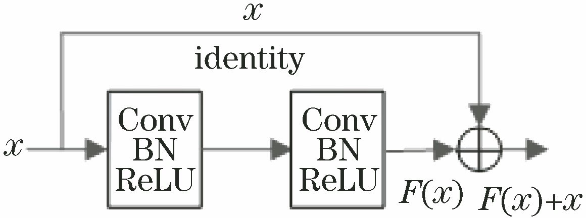
Fig. 1. Structure of residual block
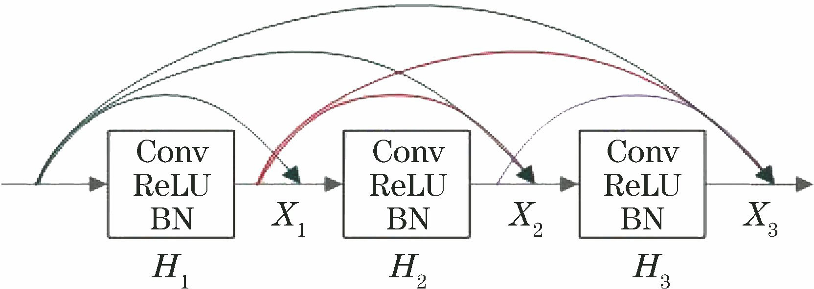
Fig. 2. Structure of dense block (l=3)
Fig. 3. Illustration of residual dense block
Fig. 4. Illustration of residual dense network model for hyperspectral image classification
Fig. 5. Classification accuracies of models with different kernel numbers
Fig. 6. Classification accuracies of models with different batch sizes
Fig. 7. Classification maps for Indian Pines dataset
Fig. 8. Classification maps of University of Pavia dataset
Fig. 9. Classification maps of Salinas dataset
Fig. 10. Classification accuracies for different training sample numbers
| Number | 1 | 2 | 3 | 4 | 5 | 6 | 7 | 8 | 9 | 10 |
|---|
| Category | Corn-notill | Corn-mintill | Grass-pasture | Grass-trees | Hay-windowed | Soybean-notill | Soybean-mintill | Soybean-clean | Woods | Total | | Number oftraining sample | 200 | 200 | 200 | 200 | 200 | 200 | 200 | 200 | 200 | 1800 | | Number oftesting sample | 1228 | 630 | 283 | 530 | 278 | 772 | 2255 | 393 | 1065 | 7434 |
|
Table 1. Numbers of Indian Pines data samples
| Number | 1 | 2 | 3 | 4 | 5 | 6 | 7 | 8 | 9 | |
|---|
| Category | Asphalt | Meadows | Gravel | Trees | Sheets | Bare Soil | Bitumen | Bricks | Shadows | Total | | Number of training sample | 200 | 200 | 200 | 200 | 200 | 200 | 200 | 200 | 200 | 1800 | | Number of testing sample | 6431 | 18449 | 1899 | 2864 | 1145 | 4829 | 1130 | 3482 | 747 | 40976 |
|
Table 2. Numbers of University of Pavia data samples
| Number | Category | Number of training sample | Number of testing sample |
|---|
| 1 | Baocoli_weeds_1 | 200 | 1809 | | 2 | Baocoli_weeds_2 | 200 | 3526 | | 3 | Fallow | 200 | 1776 | | 4 | Fallow_rough_plow | 200 | 1194 | | 5 | Fallow_smooth | 200 | 2478 | | 6 | Stubble | 200 | 3759 | | 7 | Celery | 200 | 3379 | | 8 | Grapes_untrained | 200 | 11071 | | 9 | Soil_vinyard_develop | 200 | 6003 | | 10 | Corn_senesced_weeds | 200 | 3078 | | 11 | Lettuce_romaine_4 weeks | 200 | 868 | | 12 | Lettuce_romaine_5 weeks | 200 | 1727 | | 13 | Lettuce_romaine_6 weeks | 200 | 716 | | 14 | Lettuce_romaine_7 weeks | 200 | 870 | | 15 | Vinyard_untrained | 200 | 7068 | | 16 | Vinyard_vertical_trellis | 200 | 1607 | | Total | 3200 | 50929 |
|
Table 3. Numbers of Salinas data samples
| Dataset | Criteria /% | SVM | CNN | ResNet | DenseNet | ResDenNet |
|---|
| OA | 86.82±1.12 | 96.09±0.46 | 97.79±0.47 | 97.92±0.11 | 98.71±0.01 | | IN | AA | 87.60±0.43 | 96.28±0.31 | 97.90±0.45 | 98.09±0.13 | 98.94±0.01 | | Kappa | 84.70±1.34 | 95.44±0.63 | 97.42±0.63 | 97.56±0.15 | 98.48±0.02 | | OA | 89.87±1.25 | 97.33±0.03 | 98.49±0.19 | 98.58±0.09 | 99.31±0.01 | | UP | AA | 89.91±0.51 | 96.55±0.04 | 98.26±0.16 | 98.43±0.07 | 99.08±0.02 | | Kappa | 87.32±1.46 | 96.48±0.06 | 98.01±0.34 | 98.13±0.16 | 99.08±0.01 | | OA | 89.66±1.18 | 92.84±0.52 | 96.39±0.54 | 96.52±0.15 | 97.91±0.02 | | SA | AA | 93.62±0.47 | 96.44±0.24 | 98.16±0.31 | 98.13±0.09 | 98.90±0.01 | | Kappa | 88.56±1.26 | 92.05±0.35 | 95.99±0.42 | 96.13±0.17 | 97.68±0.03 |
|
Table 4. Classification accuracies (mean value±variance) of experimental datasets
| Dataset | Criteria/% | Model based on IN | Model based on UP | Model self-trained |
|---|
| OA | 96.75±0.13 | 97.21±0.10 | 97.91±0.02 | | SA | AA | 98.52±0.01 | 98.67±0.01 | 98.90±0.01 | | Kappa | 96.38±0.16 | 96.90±0.12 | 97.68±0.03 |
|
Table 5. Classification accuracies (mean value±variance) of Salinas dataset
| Dataset | Type | CNN | ResNet | DenseNet | ResDenNet |
|---|
| IN | Train | 132.32 | 231.49 | 136.07 | 249.43 | | Test | 1.98 | 6.56 | 3.91 | 4.82 | | UP | Train | 94.87 | 156.80 | 192.23 | 187.68 | | Test | 12.29 | 14.44 | 17.08 | 16.89 | | SA | Train | 173.84 | 300.37 | 354.32 | 272.12 | | Test | 7.26 | 9.23 | 14.27 | 15.09 |
|
Table 6. Training and testing time for different methodss