
Qianwen Yang, Ke Zhou. Press-Plate State Recognition Based on Improved Bilinear Fine-Grained Model[J]. Laser & Optoelectronics Progress, 2021, 58(20): 2010007
- Laser & Optoelectronics Progress
- Vol. 58, Issue 20, 2010007 (2021)
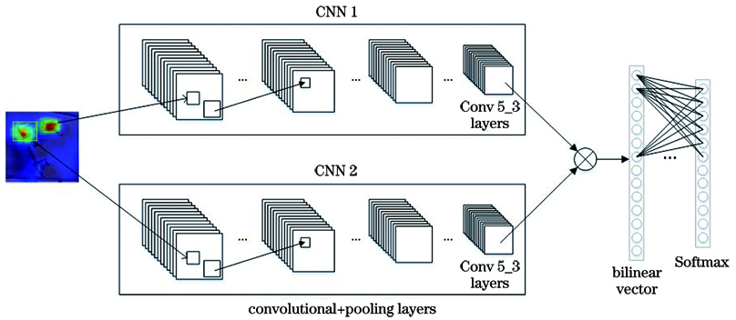
Fig. 1. Structure of the B-CNN
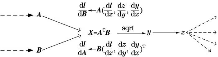
Fig. 2. Process of the gradient calculation
Fig. 3. Basic structure of the SENet
Fig. 4. Flow chart of the SENet
Fig. 5. Improved network structure
Fig. 6. Structure of the residual unit
Fig. 7. Images of press-plate in different states. (a) guan; (b) kai; (c) NS1; (d) NS2
Fig. 8. Flow chart of network training
Fig. 9. Confusion matrix of different methods. (a) Our method; (b) B-CNN
Fig. 10. Grad-CAM diagrams with different opening and closing angles of the press-plate
Fig. 11. Recognition results of different methods. (a) NS1; (b) NS2; (c) guan; (d) kai
Fig. 12. Accuracies of different methods
Fig. 13. Loss rates of different methods
Fig. 14. Accuracies of different methods in the test set
|
Table 1. Parameter of the experimental platform
|
Table 2. Initial parameters of the experiment
| |||||||||||||||
Table 3. Confusion matrix
|
Table 4. Evaluation indicators of different methods

Set citation alerts for the article
Please enter your email address
© Copyright 2018-2021 | Chinese Laser Press. All Rights Reserved 沪ICP备15018463号-20