Low-Dose CT 3D Reconstruction Using Convolutional Sparse Coding and Gradient L0-Norm

Yanqin Kang; Jin Liu; Yong Wang; Jun Qiang; Yunbo Gu; Yang Chen

doi:10.3788/AOS202141.0911005

Journals >Acta Optica Sinica >Volume 41 >Issue 9 >Page 0911005 > Article

Acta Optica Sinica
Vol. 41, Issue 9, 0911005 (2021)

Low-Dose CT 3D Reconstruction Using Convolutional Sparse Coding and Gradient L₀-Norm

Yanqin Kang^1、2, Jin Liu^1、2、*, Yong Wang¹, Jun Qiang¹, Yunbo Gu^2、3, and Yang Chen^2、3

Author Affiliations

¹College of Computer and Information, Anhui Polytechnic University, Wuhu, Anhui 241000, China

²Key Laboratory of Computer Network and Information Integration, Ministry of Education, Southeast University, Nanjing, Jiangsu 210096, China

³Laboratory of Image Science and Technology, Southeast University, Nanjing, Jiangsu 210096, China

show less

DOI: 10.3788/AOS202141.0911005 Cite this Article Set citation alerts

Yanqin Kang, Jin Liu, Yong Wang, Jun Qiang, Yunbo Gu, Yang Chen. Low-Dose CT 3D Reconstruction Using Convolutional Sparse Coding and Gradient L₀-Norm[J]. Acta Optica Sinica, 2021, 41(9): 0911005 Copy Citation Text

show less

Multi-scale online convolutional sparse coding and gradient L0 norm LDCT 3D reconstruction algorithm flow

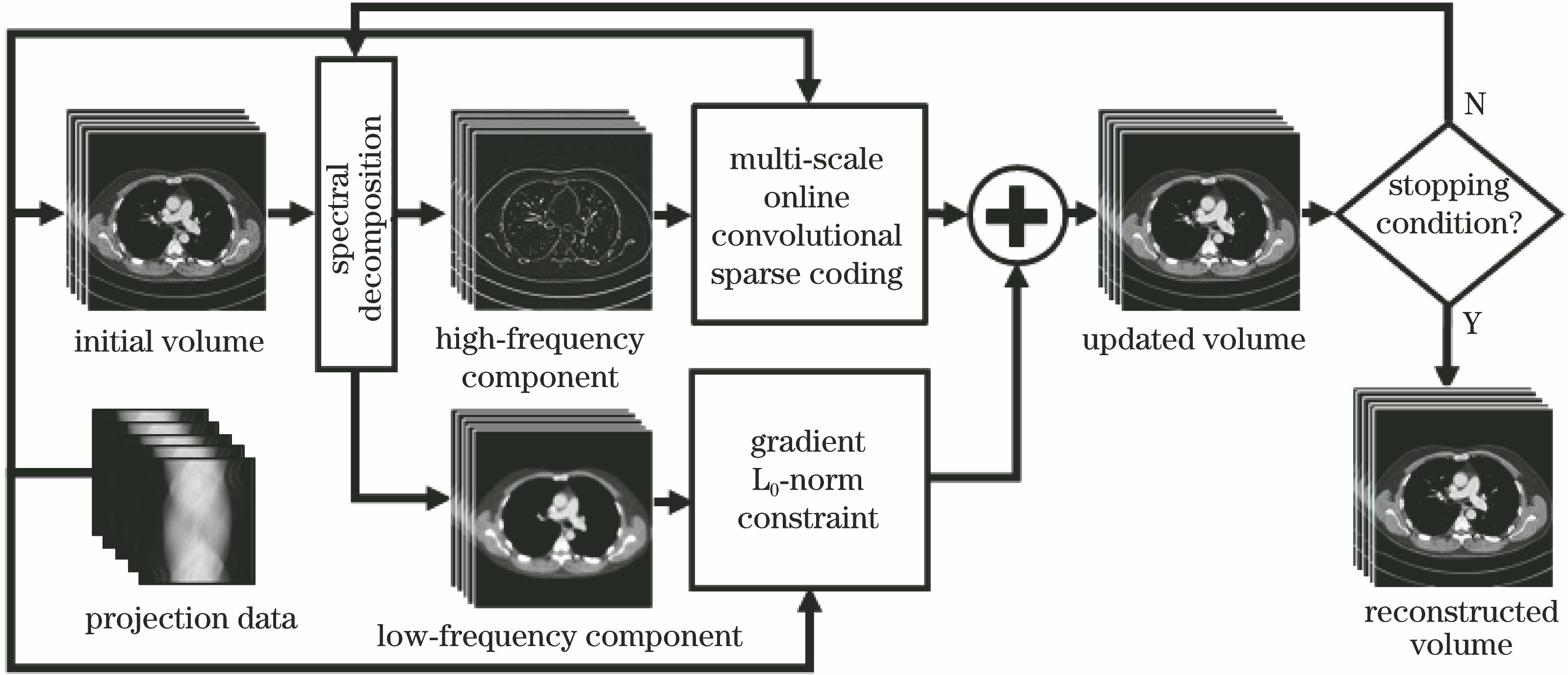
Fig. 1. Multi-scale online convolutional sparse coding and gradient L₀ norm LDCT 3D reconstruction algorithm flow

Download full size

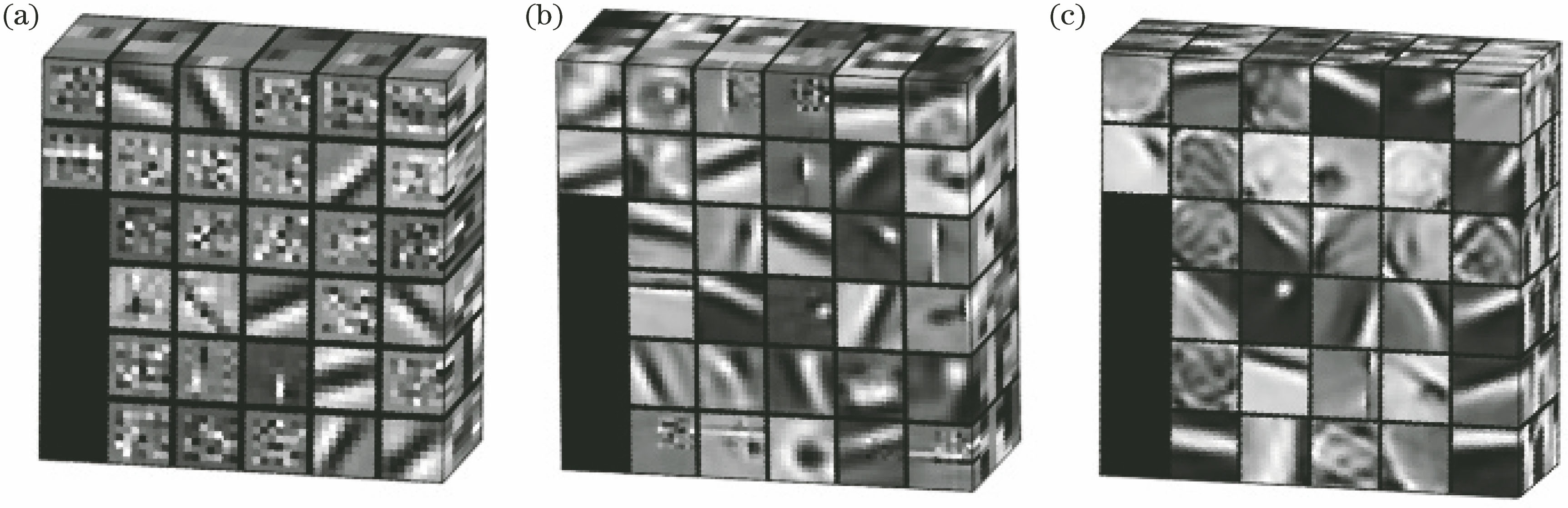
Fig. 2. 3D schematic of filter sets of different sizes after iterative convergence. (a) 8×8×4; (b) 12×12×6; (c) 16×16×8

Download full size

Fig. 3. Reconstruction results of data A under different algorithms. (a) RD-FBP algorithm; (b) LD-FBP algorithm; (c) LD-FCR algorithm; (d) LD-WCSC algorithm; (e) LD-MOCSC algorithm; (f) LD-L₀MOCSC algorithm

Download full size

Fig. 4. Reconstruction results of data B under different algorithms. (a) RD-FBP algorithm; (b) LD-FBP algorithm; (c) LD-FCR algorithm; (d) LD-WCSC algorithm; (e) LD-MOCSC algorithm; (f) LD-L₀MOCSC algorithm

Download full size

Fig. 5. NPS of reconstruction results by different algorithms. (a) LD-FBP algorithm; (b) LD-FCR algorithm; (c) LD-WCSC algorithm; (d) LD-MOCSC algorithm; (e) LD-L₀MOCSC algorithm

Download full size

Fig. 6. Reconstruction results of data C under different algorithms. (a) LD-FBP algorithm; (b) LD-FCR algorithm; (c) LD-WCSC algorithm; (d) LD-MOCSC algorithm; (e) LD-L₀MOCSC algorithm

Download full size

Fig. 7. CNR quantification results in different regions of data C reconstructed image. (a) Cross-axial slice #120; (b) coronal slice #23

Download full size

Fig. 8. Influence of simulated data on performance of L₀MOCSC algorithm under different parameters. (a) Number of different filters; (b) size of different filters

Download full size

Fig. 9. Reconstruction results of different regularization parameters. (a) λ; (b) β; (c) η; (d) γ

Download full size

Fig. 10. Performance iteration curves of different algorithms under different indexes. (a) PSNR; (b) SSIM

Download full size

Algorithm	PSNR /dB		SSIM
Algorithm	Data A	Data B	Data A	Data B
FBP	33.49±2.56	36.24±1.20	0.8016±0.0656	0.8705±0.0260
FCR	37.65±1.00	36.69±0.74	0.9066±0.0280	0.8775±0.0208
WCSC	37.84±0.51	39.66±0.68	0.9085±0.0213	0.8912±0.0206
MOCSC	37.60±0.78	39.31±0.61	0.9217±0.0241	0.9360±0.0101
L₀MOCSC	38.32±0.67	40.69±0.74	0.9288±0.0154	0.9416±0.0056

Table 1. Quantitative results of different algorithms

Algorithm		data A				data C
Algorithm		Time per iteration /s		PSNR /dB		Time per iteration /s		CNR
FCR	187±8.5		4.11		224±7.3		0.22
WCSC	144±6.1		4.34		179±6.5		0.25
MOCSC	216±5.4		4.37		291±6.4		0.32
L₀MOCSC	278±5.6		4.96		364±6.8		0.36

Table 2. Calculation time and benefits different algorithms

Yanqin Kang, Jin Liu, Yong Wang, Jun Qiang, Yunbo Gu, Yang Chen. Low-Dose CT 3D Reconstruction Using Convolutional Sparse Coding and Gradient L₀-Norm[J]. Acta Optica Sinica, 2021, 41(9): 0911005

Download Citation

Set citation alerts for the article

Tools

Set citation alerts for the article

Save the article for my favorites

Paper Information