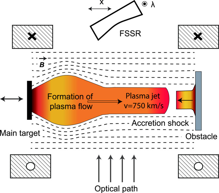
Fig. 1. Scheme (top view) of the creation of a collimated plasma stream in the laboratory (on the left) that is used to simulate the formation of an accretion column (on the right). Here, the main target is irradiated by a pulsed laser (0.6 ns/1054 nm/40 J), and then, the created plasma jet hits the solid obstacle that is used to generate accretion shocks. A magnetic field, generated by a Helmholtz coil,⁶ is applied uniformly everywhere to collimate the plasma flow.^4,6 The targets could be shifted relative to the central transverse observation hole managed in the middle of the coil system in order to observe all the expansion dynamics of the jet.^4,6 Optical and x-ray measurements (the Focusing Spectrometer with Spectral Resolution, or FSSR) are provided in the transverse direction using the observation hole. The FSSR provides spatial resolution along the whole plasma expansion axis, as well as spectral resolution in the 13–16 Å range.

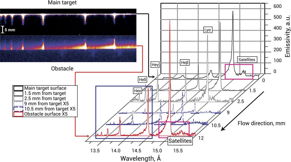
Fig. 2. Top images: measured raw data close to the main and obstacle targets; the horizontal axis is the spectral, while the vertical axis is the one along which the main plasma expansion occurs. Also shown are the spectra of fluorine lines at different distances from the laser-irradiated surface of the main target, using the FSSR spectrometer. The observed spectral components that can be used for simulating the plasma parameters are the He-series (starting with the transition 3p-1s, as highlighted in the blue box) and the Ly_α line of fluorine, with its dielectronic satellites (highlighted in the pink box).

Fig. 3. (a) Simulation of the intensity ratio for the lines He_β and He_γ using our recombination model, for different values of plasma density and temperature, compared with the experimental value of the same ratio recorded for the plasma jet stemming from the main target, i.e., the part of the plasma recorded at Z = 1 mm from a laser-irradiated target. Notably there can be, for a given plasma electron temperature, two sets of solutions: one at low density (<10¹⁸ cm⁻³) and one at high density. The solutions at low density are discarded since they are not consistent with either the density retrieved from the optical interferometric measurement, or with the hydrodynamic simulations.^4,6 (b) Solution curves in a T_e/N_e map for experimentally observed values of He_γ/He_β = 0.78, He_δ/He_β = 0.44, and He_ε/He_β = 0.16 (i.e., corresponding to the same plasma conditions at d = 1 mm from the main target), as obtained through similar calculations as those shown in (a). One can observe that using these three ratios allows a narrowing of the retrieved plasma parameters to a single solution in electron density and temperature. Here, this solution corresponds to ∼ T_e = 50 eV and N_e = 6.5 × 10¹⁸ cm⁻³. (c) and (d) Applying the same procedure at all points in the plasma along its expansion, spatial profiles of electron temperature (T_e) and density (N_e) can thus be retrieved for the case of free propagation (no obstacle and magnetic field, blue dots), for the case of jet expansion within the poloidal magnetic field of 20 T strength, with the magnetic field lines parallel to the plasma expansion (black squares), and finally, for the case of the impact on the obstacle surface, still magnetized using a 20 T magnetic field (green squares). Additionally, we give here the MHD simulation values for the electron density (green crosses), performed by the GORGON code²⁰ for the core plasma component (see below). For the shell plasma, GORGON gives N_e = 1–5 × 10¹⁸ cm⁻³ near the obstacle.

Fig. 4. Ratio of the spectral intensities of the He_γ/He_β lines for fluorine vs plasma size in the radiative-collisional code FLYCHK at 100 eV and three different electron densities (10¹⁸, 5 × 10¹⁸, 10¹⁹ cm⁻³, respectively) for optically thin and optically thick plasmas. Overlaid is the experimentally measured (using optical interferometry) range of plasma size for the considered ratios.

Fig. 5. (a) Simulation (red lines) of the experimental spectrum (black curve) using a quasi-stationary recombining model with parameters T_e = 50 eV and N_e = 2 × 10¹⁹ cm⁻³. (b) Simulation (blue lines) of the experimental spectrum (black curve) using a collisional-radiative, one-temperature model in the FLYCHK code. Note that in the model, the intensities of He-like transitions are clearly underestimated compared with what the measurements show. The experimental spectrum is recorded at the surface of the obstacle and corresponds to the configuration in which the setup is magnetized at 20 T. Please note that the spectral lines in the simulation are specially shifted in wavelength for a more convenient comparison with the experimental data.

Fig. 6. Simulation of the experimental Ly_α-to-satellites ratio for multicharged ions of fluorine as a function of electron plasma temperature. Note that the sensitivity to the density is quite low in the range of electron densities 10¹⁷–10²⁰ cm⁻³. The dielectronic satellites are located in the spectral range 15.159–15.291 Å, of which the most intense (right one inset) is F VII (2p²) ¹D₂ − (1s2p) ¹P₁. For the simulation of the Ly_α/satellites ratio, the averaged profile of all three satellites was used.

Fig. 7. Color map of electron temperature, derived by computer simulation using the GORGON code. This corresponds to the plasma near the obstacle surface (located at Z = 0), as recorded 12 ns after the incoming jet impact and for a magnetic field of 20 T. Overlaid is the comparison with x-ray data derived by the FSSR spectrometer (blue curve), following the assumption that the hotter plasma is the one in the shell. Note that the right axis pertains only to the blue curve.

Fig. 8. Simulation of the emissivity of the Ly_α line for a hot plasma component for a wide range of ion density (in units of cm⁻³) and temperature, as calculated using the FLYCHK code. The electron density is calculated each time for a given ion density and a given temperature using kinetic equations.

Table 1. X-ray spectroscopy-retrieved parameters of the two plasma components that could be identified in the experiment, simulating accretion phenomena of young stars for strengths 20 T and 6 T of the externally applied magnetic field. Here T_core and T_shell correspond to electron temperature, and N_core and N_shell to electron density, for both core and shell plasmas.