E. D. Filippov1、a), I. Yu. Skobelev1、2, G. Revet3, S. N. Chen4, B. Khiar5、6, A. Ciardi5, D. Khaghani7, D. P. Higginson3、8, S. A. Pikuz1、2, and J. Fuchs3
Abstract
Recent achievements in laboratory astrophysics experiments with high-power lasers have allowed progress in our understanding of the early stages of star formation. In particular, we have recently demonstrated the possibility of simulating in the laboratory the process of the accretion of matter on young stars [G. Revet et al., Sci. Adv. 3, e1700982 (2017)]. The present paper focuses on x-ray spectroscopy methods that allow us to investigate the complex plasma hydrodynamics involved in such experiments. We demonstrate that we can infer the formation of a plasma shell, surrounding the accretion column at the location of impact with the stellar surface, and thus resolve the present discrepancies between mass accretion rates derived from x-ray and optical-radiation astronomical observations originating from the same object. In our experiments, the accretion column is modeled by having a collimated narrow (1 mm diameter) plasma stream first propagate along the lines of a large-scale external magnetic field and then impact onto an obstacle, mimicking the high-density region of the stellar chromosphere. A combined approach using steady-state and quasi-stationary models was successfully applied to measure the parameters of the plasma all along its propagation, at the impact site, and in the structure surrounding the impact region. The formation of a hot plasma shell, surrounding the denser and colder core, formed by the incoming stream of matter is observed near the obstacle using x-ray spatially resolved spectroscopy.I. INTRODUCTION
Nowadays laser plasma is an excellent tool to simulate various magnetized supersonic and hydrodynamic flows.1–3 Recently, for example, collimated long-scaled plasma streams were used in experiments to simulate jets in Young Stellar Objects (YSOs).4 In these laboratory experiments, the most interesting processes occur far away from the laser-irradiated surface of the source target, when the plasma is no longer heated by the laser. Therefore, the common steady-state models used to analyze x-ray spectroscopy observations are not relevant, and new models geared towards recombining plasmas5 are actively being developed. This new method of x-ray spectroscopy was applied in the investigation of magnetized supersonic flows and has shown remarkable results.6
The combination of external magnetic fields and laser-produced plasmas6,7 allowed us to create a stable, collimated plasma stream which, in turn, let us investigate more complicated hydrodynamic phenomena. For example, this setup can be exploited to investigate the impact of a magnetized plasma column with an additional medium, e.g., a gas jet, solid obstacle, or another plasma. In particular, it has allowed us,8 by placing a solid obstacle in the path of the plasma column, as seen in Fig. 1, to simulate the astrophysical processes related to matter accretion onto a young star.9,10

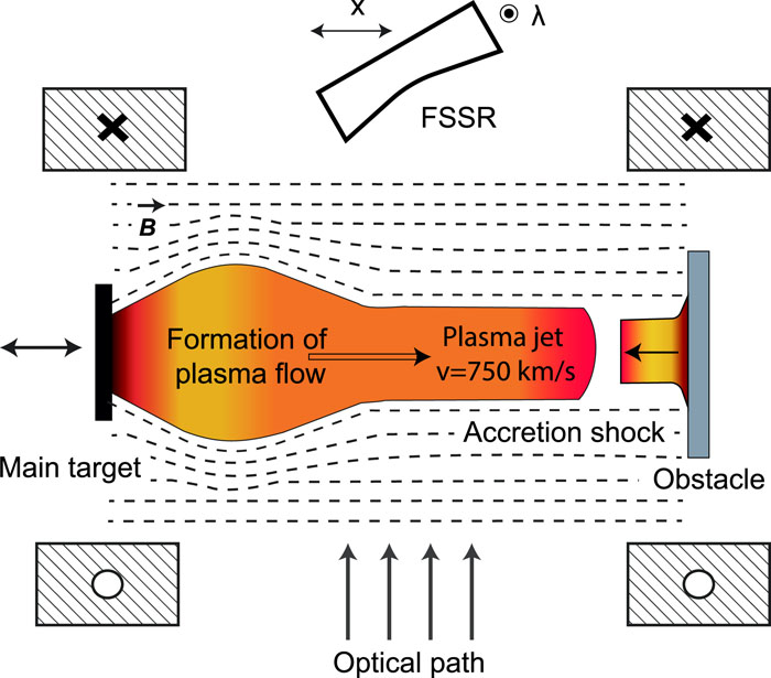
Figure 1.Scheme (top view) of the creation of a collimated plasma stream in the laboratory (on the left) that is used to simulate the formation of an accretion column (on the right). Here, the main target is irradiated by a pulsed laser (0.6 ns/1054 nm/40 J), and then, the created plasma jet hits the solid obstacle that is used to generate accretion shocks. A magnetic field, generated by a Helmholtz coil,6 is applied uniformly everywhere to collimate the plasma flow.4,6 The targets could be shifted relative to the central transverse observation hole managed in the middle of the coil system in order to observe all the expansion dynamics of the jet.4,6 Optical and x-ray measurements (the Focusing Spectrometer with Spectral Resolution, or FSSR) are provided in the transverse direction using the observation hole. The FSSR provides spatial resolution along the whole plasma expansion axis, as well as spectral resolution in the 13–16 Å range.
The purpose of this paper is to describe the new approach of x-ray diagnostics we used in such experiments, and that were recently applied successfully for the tasks of the laboratory simulation of magnetized accretion columns.8
II. EXPERIMENTAL SETUP AND MEASURED DATA
The experiments dedicated to the study of accretion dynamics in Classical T Tauri Stars (CTTSs)11 were performed at the nanosecond laser facility ELFIE at Ecole Polytechnique (France). The experimental platform was described in detail in Ref. 6 and is shown in Fig. 1. A narrow, ∼1-mm diameter, and centimeter-long collimated jet was created by the interaction of a laser beam with a solid thick target in the presence of a poloidal uniform large-scale magnetic field ∼20 T.4,6 The plasma jet evolves parallel to the lines of the magnetic field and is made to interact with a solid obstacle, mimicking a stellar chromosphere (see Fig. 1).
The plasma flow strongly emits across a wide x-ray spectral range, and so, x-ray spectroscopy methods can be used for the investigation of plasma expansion as described in Refs. 5, 12, and 13. CF2 (Teflon) targets with a low mean atomic number (Zmean = 8) were chosen in respect of the given laser intensity on the target (∼1013 W/cm2), thus creating an almost fully ionized plasma. The focusing spectrometer (FSSR), which is based on a spherically bent mica crystal, with 2d = 19.9376 Å and a radius of curvature R = 150 mm, was used to analyze the x-ray emission stemming from the plasma. For this particular setup, the FSSR was implemented to measure the x-ray spectra of multicharged fluoride ions in the range 13–16 Å (800–950 eV) in the first order of reflection (see Fig. 2). The spectrometer was installed in the direction transverse to the jet expansion, providing a spatial resolution of about 350 µm along more than 12 mm of the jet.
Figure 2.Top images: measured raw data close to the main and obstacle targets; the horizontal axis is the spectral, while the vertical axis is the one along which the main plasma expansion occurs. Also shown are the spectra of fluorine lines at different distances from the laser-irradiated surface of the main target, using the FSSR spectrometer. The observed spectral components that can be used for simulating the plasma parameters are the He-series (starting with the transition 3p-1s, as highlighted in the blue box) and the Lyα line of fluorine, with its dielectronic satellites (highlighted in the pink box).
The angles in the upwards (∼5°) and lateral (∼2°) directions were small enough for us to neglect skewing of the image. This arrangement allowed us to use the spectrometer in parallel with a Mach–Zehnder-type optical interferometer, which was used to provide complementary data about the plasma dynamics, observing the plasma electron density.8 The x-ray spectra were recorded on a fluorescent detector, a TR Fujifilm Image Plate.
Typical spectral images measured in the experiment are presented in Fig. 2. The emission is composed of Bremsstrahlung, and the following spectral components of fluoride ions: Helium-like ion emission starting with the transition 3p-1s (Heβ line) and hydrogen-like ion emission with the Lyα line and its dielectronic satellites. One can observe that the spectra change significantly as a function of the distance to the surface of the laser-irradiated target, as the plasma flow expands for many millimeters during tens of ns from the laser-interaction volume. We observed dielectronic satellites to the Lyα line near the laser-irradiated target. Here the plasma temperature is sufficient to ionize inner ion shells. Further, i.e., at >1 mm from the target surface, the absolute intensities of the spectral lines decrease and the satellites disappear. In this remote region, the contribution of He-like transitions from the level with a larger main quantum number increases in the total spectrum, which is typical of a recombining plasma.14 Then, near the obstacle surface, the absolute line intensities increase again, and satellites of the Lyα line are well distinguished, while the behavior of the He-like ion emission is preserved.
The Doppler shift is negligible and is not observed in the experimental spectrum. Notably, since the plasma flow propagates laterally, with respect to the observer (Fig. 1), only a transverse Doppler shift could arise. This would yield a spectral shift of less than 10−4 Å for the plasma velocities measured in the experiment, which are in the range 100–1000 km/s.8 For the later stages of plasma expansion, when the longitudinal Doppler shift may affect spectral line broadening, the plasma velocity is estimated to be even lower, and so the total broadening is less than the instrumental line width.
Although the signal on the detector is integrated over time, in the case of a free plasma expansion (i.e., no obstacle), the flow moves with constant velocity (i.e., all acceleration processes are supposed to occur only close to the target surface) along the spatially resolved axis; reasonably good correspondence can be made between the spatial scale and temporal evolution of the plasma parameters. However, in the case when a solid obstacle is put in the way of a plasma plume, each spatial data point measured by the spectrometer should be considered as the sum of the emitted spectra: firstly, by the laser-initiated plasma, spreading towards the obstacle; and secondly, by the plasma formed after the impact of this plasma outflow on the obstacle surface. In the experiment, the ion emission, when the plasma is freely propagating (i.e., in the absence of an obstacle), is noticeably lower compared with the emission when the plasma impacts on the solid obstacle. This means that plasma emission occurs close to the obstacle, mainly following the impact of the plasma stream on the obstacle surface.
In addition, the plasma near the obstacle consists of ions generated from both the main and obstacle targets, obfuscating their respective ion emission. One way to circumvent this issue is to use different target materials for the main and obstacle targets, such that the ions from both materials emit in different spectral ranges, which allows the separation of their emissions. This was done in our experiment using CF2 for one target and polyvinyl chloride [PVC (C2H3Cl)n] for the other.8
III. DATA ANALYSIS
The absolute and relative intensities of several spectral lines belonging to the different ionic charge states, such as those shown in Fig. 2, can be used to retrieve the plasma parameters (e.g., electron temperature and density) throughout the whole plasma expansion, and to unfold the whole scenario of the plasma-obstacle interaction.
First, one can observe that the most intense emission is located near the laser-irradiated target, since that plasma is characterized by the highest electron density, i.e., the critical density where the laser-matter interaction takes place, with Ne ∼ 1021 cm−3. The possibility of simultaneously observing the resonance lines of multiply charged K-ions and their satellites in this region is a consequence of the population and decay processes for the resonance and autoionizing levels. The satellites are initiated here by dielectronic recombination from the doubly excited states of ions which are situated very close to the corresponding resonance line (Lyα in this case). They proved to be an effective method15,16 of plasma diagnostics, since the satellite-to-resonance-line intensity ratio is essentially dependent on temperature, and in some cases on electron density. In a previous experiment conducted with identical parameters of laser and target,17 the temperature, ∼300 eV, was measured at the target surface using a steady-state plasma approach. Calculations to support inferring such a temperature were performed using the “zero-dimensional” program code FLYCHK,12 which features a collisional-radiative model.
Second, we note that the ion emission of the expanding plasma has a recombination behavior14 in the regions that are remote from the target surface. Here, at a distance >1 mm, ionization processes are negligible, and the relative intensities of the He-like spectral lines are changed due to the strong dependence of the population coefficients on the plasma parameters, as illustrated in Fig. 3(a). In general, this regime is time-dependent and not steady-state, but a quasi-stationary approach5 is commonly applied to measure plasma parameters. The approach is based on the calculation of the relative intensities of the spectral lines for ions having the same charge state [see Fig. 3(a)]. The method is sensitive to densities in the range 1016–1020 cm−3, when the temperature ranges from 10 to 100 eV for ions with Z ∼ 10; note that here we assume that the ion mean charge is “frozen.” Here the relative intensities of the 1snp1P1 − 1s21S0 transitions in the fluoride ions, where n = 3 − 7 (Heβ, Heγ, Heδ, Heε, Heξ lines correspondingly), were considered. Despite a certain error in the measurement of the intensity ratios [quantified by the width of the bar in Fig. 3(a)], the utilization of several ratios inside the He-like ion series makes it possible to unambiguously determine the electron temperature and density at any point along the plasma expansion, as illustrated in Fig. 3(b). Finally, the retrieved plasma parameters for the plasma expanding from the main target are summarized in Figs. 3(c)–3(d).
Figure 3.(a) Simulation of the intensity ratio for the lines Heβ and Heγ using our recombination model, for different values of plasma density and temperature, compared with the experimental value of the same ratio recorded for the plasma jet stemming from the main target, i.e., the part of the plasma recorded at Z = 1 mm from a laser-irradiated target. Notably there can be, for a given plasma electron temperature, two sets of solutions: one at low density (<1018 cm−3) and one at high density. The solutions at low density are discarded since they are not consistent with either the density retrieved from the optical interferometric measurement, or with the hydrodynamic simulations.4,6 (b) Solution curves in a Te/Ne map for experimentally observed values of Heγ/Heβ = 0.78, Heδ/Heβ = 0.44, and Heε/Heβ = 0.16 (i.e., corresponding to the same plasma conditions at d = 1 mm from the main target), as obtained through similar calculations as those shown in (a). One can observe that using these three ratios allows a narrowing of the retrieved plasma parameters to a single solution in electron density and temperature. Here, this solution corresponds to ∼ Te = 50 eV and Ne = 6.5 × 1018 cm−3. (c) and (d) Applying the same procedure at all points in the plasma along its expansion, spatial profiles of electron temperature (Te) and density (Ne) can thus be retrieved for the case of free propagation (no obstacle and magnetic field, blue dots), for the case of jet expansion within the poloidal magnetic field of 20 T strength, with the magnetic field lines parallel to the plasma expansion (black squares), and finally, for the case of the impact on the obstacle surface, still magnetized using a 20 T magnetic field (green squares). Additionally, we give here the MHD simulation values for the electron density (green crosses), performed by the GORGON code20 for the core plasma component (see below). For the shell plasma, GORGON gives Ne = 1–5 × 1018 cm−3 near the obstacle.
Note that, in order to apply this quasi-stationary approach, the plasma must be optically thin under laboratory conditions. An estimation of the influence of the optical depth on the intensity of ion emission can be provided by means of a comparison of the relative intensities of the 1snp1P1 − 1s21S0 transitions in the fluoride ions for optically thin and optically thick plasmas, while varying plasma size in the simulation, as illustrated in Fig. 4. In the optically thin case, the ratios of the corresponding spectral lines evidently do not depend on plasma thickness. Figure 4 gives the simulated ratio of the intensities of the spectral lines Heβ and Heγ in a plasma at Te ∼ 100 eV, with a variable density, corresponding to typical values recorded in the experiment, in the case of a recombining plasma, i.e., far from the main target [see Fig. 3(d)].17 These calculations are made for various lateral plasma sizes, using the FLYCHK code in the cases of optically thin (dashed lines) and thick plasmas (solid lines). Moreover, the experimentally measured range for the considered ratio is shown. In the experiment, the optical measurements allow4,6 us to assess the lateral size of the recombining plasma to be about 1 mm for a density ∼ 1018 cm−3. As a consequence, what can be observed in Fig. 4 is that the measured ratio is quite consistent with the one calculated in the hypothesis of an optically thin plasma. Hence, this tends to give support to the optically thin plasma hypothesis for the considered recombining plasma.
Figure 4.Ratio of the spectral intensities of the Heγ/Heβ lines for fluorine vs plasma size in the radiative-collisional code FLYCHK at 100 eV and three different electron densities (1018, 5 × 10¹⁸, 1019 cm−3, respectively) for optically thin and optically thick plasmas. Overlaid is the experimentally measured (using optical interferometry) range of plasma size for the considered ratios.
In Figs. 3(c) and 3(d), one observes a fast decrease of Te and Ne along the expansion axis in the case where no magnetic field is applied (blue dots). Conversely, in the case where we apply a magnetic field of 20 T strength (black dots), the initially heated plasma flow maintains itself far from the main target; i.e., at distances >2 mm, almost constant values of electron temperature and density exist, i.e., Te ∼ 20 eV and Ne ∼ 4 × 1018 cm−3 respectively. When an obstacle is put in the way of the plasma propagation (green dots), we observe a substantial increase in the electron temperature and density, up to 50 eV and 2 × 1019 cm−3, respectively, in the region near the obstacle.
To retrieve the plasma parameters in the case when a solid unheated obstacle is put in the way of the recombining plasma, one has to carefully consider that the shock formation and plasma heating at the location of the obstacle can lead to an additional excitation of ions. Typically, this implies higher temperatures (Te ≫ 100 eV, exceeding the ionization potential for the L-shell) and higher densities than in the free propagation case.18,19 Here, the recombination approach alone is no longer applicable, and an additional contribution to the kinetic model by ionization should be taken into account. Figure 5(a) demonstrates the sudden appearance of a strong Lyα line, as well as satellites near the obstacle position, both of which definitely cannot be described using solely a recombination model [as shown by the red lines in Fig. 5(a)]. The spectra shown here were integrated over 400 µm along the expansion axis to achieve a better signal-to-noise ratio. As can be seen in Fig. 5(b), a simulation performed in a steady-state collisional-radiative model with a single-temperature plasma fits the experimental ratio Lyα/Heβ, as well as describing the satellites nearby; however, the intensities of the other He-like lines, with a larger main quantum number n, are clearly underestimated. Thus, according to Fig. 5(a), a reasonable assumption is to assume the presence of an additional plasma component, in addition to the one modeled in Fig. 5(a), which can yield the observed strong Lyα line. The observed x-ray emission stemming from near the obstacle surface can thus be envisioned as resulting from the overlap of two emissions originating from two different plasmas. The first emission originates from the recombining plasma coming from the main target which has propagated up to the obstacle, while the second emission, contributing to the observed higher charge states (Lyα and satellites), comes from a hotter plasma generated at the obstacle surface, following the impact of the expanding jet. This latter emission can be described by a pure steady-state model.
Figure 5.(a) Simulation (red lines) of the experimental spectrum (black curve) using a quasi-stationary recombining model with parameters Te = 50 eV and Ne = 2 × 1019 cm−3. (b) Simulation (blue lines) of the experimental spectrum (black curve) using a collisional-radiative, one-temperature model in the FLYCHK code. Note that in the model, the intensities of He-like transitions are clearly underestimated compared with what the measurements show. The experimental spectrum is recorded at the surface of the obstacle and corresponds to the configuration in which the setup is magnetized at 20 T. Please note that the spectral lines in the simulation are specially shifted in wavelength for a more convenient comparison with the experimental data.
Hence, the experimental spectrum was simulated using the electron temperature and density, according to the experimental x-ray data: T1 = 50 eV, N1 = 2.3 × 10¹⁹ сm−3 for the shocked plasma, modeled by a recombining model; T2 = (320–600) eV for the shocked plasma near the obstacle, using the simulation of Lyα to satellites (see Fig. 6) in a steady-state model. The satellites have a low intensity in the experimental data, and so, the method based on analyzing their relative intensity to that of the Lyα line produces significant error, represented in Fig. 6 by the rectangular hatching. Note that this uncertainty in the measurement also hampers us in determining reliable values for the density of the second plasma component, which is why it is not quoted here.
Figure 6.Simulation of the experimental Lyα-to-satellites ratio for multicharged ions of fluorine as a function of electron plasma temperature. Note that the sensitivity to the density is quite low in the range of electron densities 1017–1020 cm−3. The dielectronic satellites are located in the spectral range 15.159–15.291 Å, of which the most intense (right one inset) is F VII (2p2) 1D2 − (1s2p) 1P1. For the simulation of the Lyα/satellites ratio, the averaged profile of all three satellites was used.
Notably, the plasma parameters inferred in this way for the two components of the plasma near the obstacle surface are very consistent with the simulated results using the GORGON20 code; evidence is found of the formation of a hot plasma “shell” surrounding a central, colder “core” [see Figs. 7 and 3(d)]. Here the terms “hot” and “cold” refer to electron temperature only. The hot shell observed in the GORGON simulation is consistent with the plasma component that yields the strong Lyα line and the associated satellites. The model used in the GORGON simulation describes a two-temperature, one-fluid resistive plasma which is optically thin. The model was initially developed for experiments in Z-pinches but is now widely used for laboratory astrophysics laser-plasma experiments.21,22 The formation of the hot (in terms of electron plasma temperature) shell, as observed in the simulation performed using the GORGON code, results from the following scenario: after the laser-induced plasma stream has impacted the obstacle, the shocked plasma escapes radially but is recollimated on-axis by the external magnetic field. This recollimation of the plasma flow is accompanied by heating of the electrons within the peripheral regions, i.e., in the shell.8 Indeed, within the core, there is a decoupling of the ion and electron temperatures after the shock, the ions being the ones heated by the shock. Since the electrons can only be heated through collisions along their trajectories, given sufficient time, hot electrons are predominantly located in the shell.
Figure 7.Color map of electron temperature, derived by computer simulation using the GORGON code. This corresponds to the plasma near the obstacle surface (located at Z = 0), as recorded 12 ns after the incoming jet impact and for a magnetic field of 20 T. Overlaid is the comparison with x-ray data derived by the FSSR spectrometer (blue curve), following the assumption that the hotter plasma is the one in the shell. Note that the right axis pertains only to the blue curve.
Thus, the x-ray spectra shown in Fig. 5 describe two plasma components separated in space: one is a plasma shell and the other is a plasma core. Since we have already been able to derive the parameters of the cold core, we will now focus on ascertaining the density of the hot shell (the temperature of the latter was already inferred by the Lyα/satellites ratio, see Fig. 6). For this, we will focus on the ratio between the Lyα and Heβ lines in the x-ray spectra, since the hydrogen and helium–like series for a given spectral range belong mostly to different plasma components. The He-like series of ion emission is emitted by the recombining plasma (i.e., the cold core), while the Lyα line is mainly produced by the hot post-shocked zone (i.e., in the shell). The emissivity of the hot plasma can be evaluated for a wide range of electron densities (see Fig. 8) by a steady-state model in FLYCHK. The emissivity of the He-like emission, in contrast, is defined using a quasi-stationary approach.5 Here, the experimentally observed ratio can be expressed aswhere E is the emissivity of a spectral line, V the volume of a corresponding plasma component, and the emissivity, , is calculated by a recombination model.5 Taking the volume ratio between the two plasma (shell/core) fractions retrieved from the interferometry data,8 it is possible to calculate the electron density of the hot plasma (i.e., the shell) component in the experiment as being up to ∼5 × 1018 cm−3.
Figure 8.Simulation of the emissivity of the Lyα line for a hot plasma component for a wide range of ion density (in units of cm−3) and temperature, as calculated using the FLYCHK code. The electron density is calculated each time for a given ion density and a given temperature using kinetic equations.
The final parameters of the plasma components for the magnetic field strengths used in the experiment, 20 T and 6 T, are depicted in Table I. Note that, in the latter case, the analysis was performed according to what has been detailed above. Here, in line with the GORGON simulations and the optical interferometry data,8 we have assumed that the hot plasma component is a shell enveloping a cold core. We observe a significant difference between the 20 T and 6 T cases, in terms of electron densities, for the core plasma, up to ∼10 times; note that such a difference is fully consistent with optical interferometry data. Moreover, the electron temperature is similar for both cases. We associate this effect with the additional ionization of plasma and collimation of plasma flow when the magnetic field is applied. This leads to the increase in plasma density and the faster recombination rate, making it possible to measure the electron density using our technique.
| B field (T) | Tcore (eV) | Ncore (cm−3) | Tshell (eV) | Nshell (cm−3) |
|---|
| 20 | 50 | 2.3 × 10¹⁹ | 320–600 | 3.8–4.9 × 10¹⁸ |
| 6 | 40 | 3.3 × 10¹⁸ | 320–600 | 3.7–4.6 × 10¹⁷ |
Table 1. X-ray spectroscopy-retrieved parameters of the two plasma components that could be identified in the experiment, simulating accretion phenomena of young stars for strengths 20 T and 6 T of the externally applied magnetic field. Here Tcore and Tshell correspond to electron temperature, and Ncore and Nshell to electron density, for both core and shell plasmas.
For the shell, its optical depth can be evaluated in FLYCHK, in a similar way to what was done for the recombining plasma (i.e., the core), as presented in Fig. 4. The value of the optical depth is found here to be τ ∼ 0.3, validating, a posteriori, the possibility of using the Lyα to Heβ ratio for evaluating the shell plasma parameters. Even though we note that the shell revealed in the experiment is optically thin, we have to note that this is not necessarily so in the astrophysical case; i.e., the transport of x-ray emission is not scalable from the laboratory to the astrophysical case. For example, strong emission in the x-ray and UV ranges is suggested to take place following the impact of accretion columns on YSOs, due to the high temperature induced in the shocked plasma.23 However, recent astrophysical observations24,25 have shown that the mass-accretion rates are different for calculations based on x-ray and optical ranges of radiation. The effect of the optical depth in the x-ray range is given as one possible reason. The explanation can be also found in Ref. 26 where the idea of an “accretion-fed corona” is presented. In that case, the x-ray emission originates from three plasma components: a hot corona; a high-density, post-shock region close to the shock front; and a cold, less-dense, post-shock cooling region. We stress here that in the astrophysical case,26 the situation, in terms of electron temperature, is the reverse of the situation observed in the laboratory, namely one of a cold shell surrounding a hot core. This is due to the very short equilibration time between ions and electrons in the astrophysical case compared with the time-scale of hydrodynamic-shell formation; in contrast, in the laboratory experiment, shell formation takes place on shorter time scales than the ions’ and electrons’ equilibration. Hence, the formation of a cold-shell plasma, highlighted here in laboratory experiments, could, in the astrophysical case, potentially lead to x-ray absorption of the emission originating from the hot core, directly influencing the calculated mass-accretion rate.
IV. CONCLUSIONS
We developed a combined approach to characterize the dynamics of a magnetized plasma flow when it collides with a solid obstacle, mimicking the formation of accretion columns in young stars. The approach is based on the simulation of the relative intensities of x-ray spectral lines emitted by differently charged ionic states. On top of the plasma flow colliding onto the obstacle, a shock develops in which the ions are first heated, and hence, the electrons stay relatively cold. We assume the generation of an additional, hotter plasma component that results from the expansion into vacuum of the plasma escaping from the shock region. That second plasma component induces a significant x-ray emission from higher charge states, i.e., the Lyα line and its dielectronic satellites. The ratio between the emitted Lyα and Heβ lines in the x-ray region was successfully used to derive the localization of these two plasma components, since these two lines are predominantly emitted by the hotter (post-shock) and colder (shocked) plasma components, respectively. Overall, this leads to evidence for the formation of a hot plasma shell with Te > 320 eV, enveloping a cold, dense core with Te ∼ 50 eV and Ne ∼ 2 × 1019 cm−3. These plasma parameters are consistent with numeric simulations performed by the magnetohydrodynamic code GORGON and with optical interferometry measurements of the same plasma.8 The formation of shell plasma in the astrophysical case could lead to substantial absorption of x-ray emission of accretion columns generated in YSOs.8
References
[1] Y. T. Li, D. W. Yuan, B. Q. Zhu, J. Q. Zhu, Z. Zhang, C. Wang, G. Y. Liang, J. M. Peng, B. J. Zhu, G. Y. Hu, H. G. Wei, W. M. Jiang, B. Han, X. W. Ma, J. Y. Zhong, X. Gao, J. Zhang, T. Tao, G. Zhao, F. L. Wang. Laboratory analog of heavy jets impacting a denser medium in herbig–haro (HH) objects. Astrophys. J., 868, 56(2018).
[2] R. Betti, T. C. Sangster, R. K. Follett, P. A. Amendt, D. Lamb, D. D. Ryutov, D. H. Froula, A. Frank, H. Sio, B. A. Remington, P. A. Norreys, G. Gregori, S. X. Hu, P. Tzeferacos, R. P. Drake, N. C. Woolsey, P. Hartigan, M. J. Rosenberg, H. G. Rinderknecht, J. A. Frenje, C. C. Kuranz, S. C. Wilks, R. D. Petrasso, M. Koenig, C. K. Li, A. B. Zylstra, S. V Lebedev, F. H. Seguin, H. S. Park. Scaled laboratory experiments explain the kink behaviour of the Crab Nebula jet. Nat. Commun., 7, 13081(2016).
[3] E. Falize, R. Sweeney, B. Loupias, S. Klein, R. P. Drake, M. Grosskopf, C. C. Kuranz, R. Gillespie, C. M. Krauland, P. A. Keiter. Radiative reverse shock laser experiments relevant to accretion processes in cataclysmic variables. Phys. Plasmas, 20, 056502(2013).
[4] F. Kroll, J. Fuchs, L. Romagnani, G. Revet, A. Soloviev, A. Ciardi, H.-P. H.-P. Schlenvoigt, M. Nakatsutsumi, C. Riconda, S. N. Chen, M. Huarte-Espinosa, M. Huarte-Espinosa, K. Naughton, I. Y. Skobelev, O. Portugall, J. Fuchs, J. Béard, R. Riquier, T. Herrmannsdörfer, T. Herrmannsdorfer, H. Pépin, G. Revet, S. A. Pikuz, T. Vinci, Z. Burkley, F. Kroll, S. A. Pikuz, D. P. Higginson, J. Beard, O. Portugall, B. Albertazzi, C. Riconda, A. Y. Y. Faenov, M. Borghesi, K. Naughton, H.-P. H.-P. Schlenvoigt, J. Billette, I. Y. Skobelev, A. Y. Y. Faenov, S. N. Chen, A. Soloviev, A. Frank, R. Bonito, R. Riquier, T. E. Cowan, J. Billette, H. Pepin, D. P. Higginson, R. Bonito, L. Romagnani, M. Borghesi, A. Frank, T. E. Cowan, Z. Burkley. Laboratory formation of a scaled protostellar jet by coaligned poloidal magnetic field. Science, 346, 325(2014).
[5] I. Y. Skobelev, A. Y. Faenov, S. A. Pikuz, T. A. Pikuz, A. N. Grum-Grzhimailo, S. N. Ryazantsev. X-ray spectroscopy diagnostics of a recombining plasma in laboratory astrophysics studies. JETP Lett., 102, 707(2015).
[6] T. Vinci, M. Blecher, B. Khiar, D. Khaghani, M. Starodubtsev, K. Burdonov, S. N. Ryazantsev, K. Naughton, O. Willi, M. Borghesi, C. Riconda, D. P. Higginson, J. Fuchs, G. Revet, I. Y. Skobelev, S. Pikuz, H. Pépin, S. N. Chen, E. Filippov, R. Riquier, J. Béard, A. Soloviev, O. Portugall, A. Ciardi. Detailed characterization of laser-produced astrophysically-relevant jets formed via a poloidal magnetic nozzle. High Energy Density Phys., 23, 48(2017).
[7] J. Fuchs, V. Tikhonchuk, J. Béard, R. Riquier, H. Pépin, B. Pollock, S. N. Chen, P. Korneev, S. Pikuz, D. P. Higginson, E. D’Humières. A novel platform to study magnetized high-velocity collisionless shocks. High Energy Density Phys., 17, 190(2015).
[8] R. Rodriguez, A. Ciardi, O. Portugall, K. Naughton, H. Pépin, M. Borghesi, O. Willi, S. Pikuz, R. Bonito, E. Filippov, S. Orlando, M. Blecher, G. Revet, S. N. Chen, R. Riquier, A. Soloviev, K. Burdonov, C. Argiroffi, D. Khaghani, D. P. Higginson, J. Fuchs, I. Yu. Skobelev, J. Béard, B. Khiar, S. N. Ryazantsev. Laboratory unraveling of matter accretion in young stars. Sci. Adv., 3, e1700982(2017).
[9] C. Knigge, S. Scaringi, T. J. Maccarone, S. Vaughan, S. C. C. Barros, E. Kording, E. Aranzana, T. R. Marsh, V. S. Dhillon. Accretion-induced variability links young stellar objects, white dwarfs, and black holes. Sci. Adv., 1, e1500686(2015).
[10] W. J. De Wit, T. P. Ray, L. Moscadelli, A. Caratti O Garatti, R. D. Oudmaijer, B. Stecklum, J. Greiner, R. Garcia Lopez, R. Cesaroni, A. Sanna, C. Fischer, J. M. Ibañez, R. Klein, A. Krabbe, C. M. Walmsley, J. Eislöffel. Disk-mediated accretion burst in a high-mass young stellar object. Nat. Phys., 13, 276(2017).
[11] G. G. Sacco, C. Argiroffi, F. Reale, A. Maggio, S. Orlando. X-ray emitting MHD accretion shocks in classical T Tauri stars. Case for moderate to high plasma-beta values. Astron. Astrophys., 510, A71(2010).
[12] R. W. Lee, M. H. Chen, Y. Ralchenko, W. L. Morgan, H. K. Chung. FLYCHK: Generalized population kinetics and spectral model for rapid spectroscopic analysis for all elements. High Energy Density Phys., 1, 3(2005).
[13] I. E. Golovkin, R. B. Campbell, D. R. Welch, B. V Oliver, J. J. MacFarlane, P. R. Woodruff, T. A. Mehlhorn. Simulation of the ionization dynamics of aluminum irradiated by intense short-pulse lasers(2003).
[14] I. Y. Skobelev, A. Y. Faenov, F. B. Rosmej. High resolution X-ray spectroscopy of laser generated plasmas. Phys. Scr. T, 80, 43(1999).
[15] A. H. Gabriel. Dielectronic satellite spectra for highly-charged helium-like ion lines. Mon. Not. R. Astron. Soc., 160, 99(1972).
[16] Y. Li, J. Zhu, J. Zhao, G. Liang, J. Zhang, C. Wang, N. Hua, J. Zhong, F. Wang, C. Liu, B. Han, F. Li, D. Yuan, H. Wei, Y. Li, B. Zhu, G. Jia, Z. Zhang, J. Xiong, G. Zhao. Measurement and analysis of K-shell lines of silicon ions in laser plasmas. High Power Laser Sci. Eng., 6, e31(2018).
[17] S. A. Pikuz, S. N. Chen, J. Fuchs, D. Khaghani, D. P. Higginson, I. Y. Skobelev, G. Revet, E. D. Filippov, S. N. Ryazantsev. Parameters of supersonic astrophysically-relevant plasma jets collimating via poloidal magnetic field measured by x-ray spectroscopy method. J. Phys.: Conf. Ser., 774, 012114(2016).
[18] A. P. Shevelko, L. P. Presnyakov, I. L. Beigman, D. B. Uskov, P. Y. Pirogovskiy. Interaction of a laser-produced plasma with a solid surface: Soft X-ray spectroscopy of high-Z ions in a cool dense plasma. J. Phys. B: At., Mol. Opt. Phys., 22, 2493(1989).
[19] L. P. Presnyakov, M. A. Mazing, P. Y. Pirogovskiy, A. P. Shevelko. Interaction of a laser-produced plasma with a solid surface. Phys. Rev. A, 32, 3695(1985).
[20] G. N. Hall, T. Lery, E. G. Blackman, J. Rapley, J. P. Chittenden, C. Stehle, D. J. Ampleford, F. A. Suzuki-Vidal, C. J. Jennings, S. C. Bott, S. N. Bland, A. Ciardi, A. Frank, A. Marocchino, S. V. Lebedev. The evolution of magnetic tower jets in the laboratory. Phys. Plasmas, 14, 056501(2007).
[21] L. Romagnagni, S. Nitsche, M. Nakatsutsumi, S. N. Chen, H. Pépin, J. Fuchs, S. Simond, O. Portugall, B. Hirardin, A. Ciardi, T. E. Cowan, J. Béard, B. Albertazzi, H. P. Schlenvoigt, E. Veuillot, D. Da Silva, S. Dittrich, T. Burris-Mog, F. Kroll, J. Billette, C. Riconda, T. Vinci, J. Albrecht, T. Herrmannsdörfer. Production of large volume, strongly magnetized laser-produced plasmas by use of pulsed external magnetic fields. Rev. Sci. Instrum., 84, 043505(2013).
[22] J. Fuchs, B. Albertazzi, O. Portugall, H. Pépin, C. Riconda, T. Vinci, A. Ciardi. Astrophysics of magnetically collimated jets generated from laser-produced plasmas. Phys. Rev. Lett., 110, 025002(2013).
[23] P. J. Armitage. Dynamics of protoplanetary disks. Annu. Rev. Astron. Astrophys., 49, 195(2011).
[24] G. Peres, J. J. Drake, C. Argiroffi, S. Sciortino, B. Stelzer, J. L. Santiago, A. Maggio. X-ray optical depth diagnostics of T Tauri accretion shocks. Astron. Astrophys., 507, 939(2009).
[25] R. L. Curran, C. Argiroffi, G. G. Sacco, G. Peres, S. Orlando, F. Reale, A. Maggio. Multi-wavelength diagnostics of accretion in an X-ray selected sample of CTTSs. Astron. Astrophys., 526, 104(2011).
[26] S. R. Cranmer, N. S. Brickhouse, S. Wolk, G. J. M. Luna, A. K. Dupree. A deep Chandra X-ray spectrum of the accreting young star TW Hydrae. Astrophys. J., 710, 1835(2010).