Time-energy analysis of the photoionization process in a double-XUV pulse combined with a few-cycle IR field

Yi Jia; Li Guo; Shilin Hu; Xinyan Jia; Daihe Fan; Ronghua Lu; Shensheng Han; Jing Chen

doi:10.3788/COL202119.123201

Abstract

We calculate the time-energy distribution (TED) and ionization time distribution (ITD) of photoelectrons emitted by a double-extreme-ultraviolet (XUV) pulse and a two-color XUV-IR pulse using the Wigner distribution-like function based on the strong field approximation. For a double-XUV pulse, besides two identical broad distributions generated by two XUV pulses, many interference fringes resulting from the interference between electrons generated, respectively, by two pulses appear in the TED. After adding an IR field, the TED intuitively exhibits the effect of the IR field on the electron dynamics. The ITDs during two XUV pulses are no longer the same and show the different changes for the different two-color fields, the origin of which is attributed to the change of the electric field induced by the IR field. Our analysis shows that the emission time of electrons ionized during two XUV pulses mainly depends on the electric field of the combined XUV pulse and IR pulse.

Keywords

attosecond physics strong field approximation time-energy distribution two-color field Wigner distribution

1. Introduction

The generation of the ultrashort optical pulses in the extreme ultraviolet (XUV) range has allowed the electron’s ultrafast dynamic processes in atoms^[1–5], molecules^[6–8], and solids^[9–11] to be studied on the attosecond (as, 1 as $= 10^{- 18} s$ ) timescale. High-order harmonic generation (HHG)^[12,13] is the primary method to obtain as XUV pulses when an infrared (IR) pulse interacts with the atoms. A long IR laser pulse leads to an as pulse train (APT)^[14,15]. A single as pulse (SAP)^[16–18] can be obtained using a few-cycle IR pulse. Generally, it is easier to produce an APT experimentally than an isolated XUV pulse.

An as XUV pulse train or a single XUV pulse is widely applied to investigate as time delays of photoemission when they are combined with a phase-locked IR field. When an as train is combined with an IR field, this scheme is often referred to as the reconstruction of as beating by interference of two-photon transition (RABBITT)^[19] method. The as streaking technique refers to an as pulse in the presence of an IR field^[20]. Based on the RABBITT technique, Klünder et al.^[2] have demonstrated that the time delay between electrons emitted from the $3 p$ and $3 s$ orbitals in argon atom is 110 as. Schultze et al.^[21] have obtained a time delay of $\sim 21$ as in the emission of electrons liberated from the $2 p$ orbital of the neon atom with respect to that released from the $2 s$ orbital at an XUV photon energy of 100 eV using as streaking technique. These two techniques can also be used to determine the basic properties of the as XUV pulse train^[19,22] and the single XUV pulse^[20].

It is known that the photoionization processes in the as streaking technique and the RABBITT technique are laser-assisted, where an electron is ionized in the superposition of the XUV and IR fields. The effect of the IR field on the electron dynamics cannot be neglected^[23–25]. In our previous work, we have investigated the effect of the IR field on the electron dynamics^[26] in the as streaking technique. We find that the IR field not only modifies the final electron kinetic energy, but also changes the electron’s emission time in the case of SAP combined with an IR field^[26]. It is worth mentioning that Cattaneo et al.^[27] have concluded that the time information extracted from the as streaking technique and the RABBITT technique is slightly different under the same condition. It is necessary to further study the effect of the IR field on the electron dynamics in the case of the RABBITT technique.

Sign up for Chinese Optics Letters TOC. Get the latest issue of Chinese Optics Letters delivered right to you！Sign up now

In this paper, we mainly study the effects of the IR field on the dynamics of the electron emitted by a double-XUV pulse alone and in the presence of an IR field using a Wigner distribution-like (WDL) function based on the strong field approximation (SFA) theory.

2. Theory Method

The first term of the $S$ -matrix element^[28] (namely, the SFA theory) is given as follows: $S_{f i} = - i \int_{- \infty}^{\infty} d t 〈 ψ_{A f} (p, t) | V_{A} | φ_{i} (t) 〉 .$ (1)

Here, $V_{A} = - r \cdot E (t)$ is the interaction potential in the length gauge. $| φ_{i} (t) 〉 = | φ_{0} 〉 e^{i I_{p} t}$ is the atomic ground state, where $I_{p}$ denotes the ionization potential. $| ψ_{A f} (p, t) 〉$ is the Volkov state with the final electron momentum $p$ , which is written as $| ψ_{A f} (p, t) 〉 = \frac{1}{\sqrt{v}} \exp {i [p + A (t)] \cdot r - i S_{p} (t)},$ (2)where $S_{p} (t) = \frac{1}{2} \int_{- \infty}^{t} {[p + A (τ)]}^{2} d τ$ , $v$ is the normalization volume, and $A (t)$ is the vector potential of the applied laser pulse.

Substituting Eq. (2) into Eq. (1), we can get $S_{f i} = \frac{- i}{\sqrt{v}} \int_{- \infty}^{\infty} d t 〈 p + A (t) | V_{A} | φ_{0} 〉 \times \exp [i S_{p} (t) + i I_{p} t] = \frac{1}{\sqrt{2 π}} \int_{- \infty}^{\infty} d t S^{'} e^{i \frac{p^{2}}{2} t},$ (3)where $| p + A (t) 〉 = e^{i [p + A (t)] \cdot r}$ , and the expression of $S^{'}$ is $S^{'} = \frac{- i \sqrt{2 π}}{\sqrt{v}} 〈 p + A (t) | V_{A} | φ_{0} 〉 \times \exp {i \int_{- \infty}^{t} [p \cdot A (τ) + \frac{A {(τ)}^{2}}{2}] d τ + i I_{p} t} .$ (4)

The detailed definition and derivation of the WDL function can be found in Refs. [29,30]. Here, we directly give the WDL function in one-dimensional system, which is written as $f (t, \frac{p^{2}}{2}, Θ) = \frac{1}{π} \int_{- \infty}^{\infty} S^{'' *} (t + t^{'}, Θ) \times S^{''} (t - t^{'}, Θ) e^{- 2 i \frac{p^{2}}{2} t^{'}} d t^{'},$ (5)where $S^{''} = S^{'} / \sqrt{p}$ . $p^{2} / 2$ is the final energy of the electron, and $Θ$ is the angle between the final electron momentum $p$ and the $x$ axis.

The WDL function satisfies the following relationship: $\int_{- \infty}^{\infty} f (t, \frac{p^{2}}{2}) d t = \frac{{| S_{f i} |}^{2}}{p} .$ (6)

The energy spectrum of photoelectrons can be given exactly by Eq. (6) in the one-dimensional system.

Further, the ionization time distribution (ITD) $P (t)$ can be obtained by integrating Eq. (5) over the final energy $p^{2} / 2$ , which is $P (t) = \int f (t, \frac{p^{2}}{2}) d (\frac{p^{2}}{2}) .$ (7)

In this paper, the vector potential of two XUV pulses in the presence of an IR field is given by $A (t) = A_{IR} (t) + A_{XUV 1} (t) + A_{XUV 2} (t) .$ (8)

Here, $A_{IR} (t) = - \frac{E_{IR}}{ω} \sin^{2} (\frac{π t}{τ_{IR}}) \cos (ω t + φ_{IR}) e_{x}, 0 < t < τ_{IR},$ (9) $A_{XUV i} (t) = - \frac{E_{XUV}}{Ω} \sin^{2} [\frac{π (t - t_{C i} + \frac{τ_{XUV}}{2})}{τ_{XUV}}] \times \cos [Ω (t - t_{C i} + \frac{τ_{XUV}}{2}) + φ_{XUV}] e_{x}, t_{C i} - \frac{τ_{XUV}}{2} < t < t_{C i} + \frac{τ_{XUV}}{2}, i = 1, 2 .$ (10)

Here, the subscripts $i = 1$ and 2 correspond to the first and second XUV pulses, respectively. $τ_{IR}$ ( $τ_{XUV}$ ), $φ_{IR}$ ( $φ_{XUV}$ ), and $ω$ ( $Ω$ ) are the pulse duration, carrier-envelope phase (CEP), and laser frequency of the IR (XUV) pulse, respectively. $E_{IR}$ ( $E_{XUV}$ ) is the peak electric field strength of the IR (XUV) pulse. In this paper, the pulse durations $τ_{IR}$ and $τ_{XUV}$ are fixed, containing four cycles. $t_{C 1}$ ( $t_{C 2}$ ) is the time corresponding to the center of the first (second) XUV pulse, and $e_{x}$ is the unit vector along the $x$ axis.

In the present work, we mainly adopt a model atom with $I_{p} = 1$ a.u. Atomic units (a.u.) are used throughout this paper unless indicated otherwise. The frequency and intensity of each XUV pulse are $Ω = 1.5$ a.u. and $I_{XUV} = 1 \times 10^{14} W / {cm}^{2}$ , respectively. The time variables are in units of optical cycles (o.c.) of the involved IR field.

3. Results and Discussions

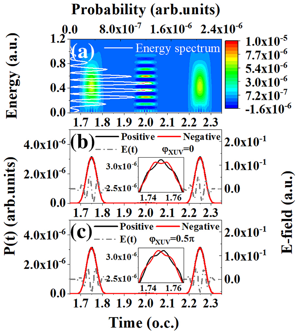
In Fig. 1(a), we first calculate the time-energy distributions (TEDs) of electrons emitted along the positive $x$ axis (called “positive direction” below) in two XUV pulses ( $φ_{XUV} = 0$ ) spaced by a half-cycle of an 800 nm IR field. It is expected that two broad distributions appear in the TED at times only when the XUV pulse is present. Meanwhile, many horizontal fringes are clearly located at the middle of two XUV pulses, which come from the constructive interference between electrons with the same energy generated, respectively, by the two XUV pulses. It is worth mentioning that the center position of the interference fringe along the time axis is fixed at the middle of the two XUV pulses, which is determined by the feature of the WDL function. The width of the interference fringe is dependent on the XUV pulse duration. On the other hand, the center position of the interference fringe along the energy axis can be approximately explained in an alternative way from the frequency domain point of view: an electron is ionized by absorbing one photon with different energy. Figure 2 presents the frequency spectrum of the double-XUV pulse with parameters as those of Fig. 1(a). Hence, the center positions of the constructive interference fringes along the energy axis can be approximately given by $\frac{p^{2}}{2} \approx Ω_{i} - I_{p}$ , where $Ω_{i}$ denotes any frequency in the frequency spectrum of the double-XUV pulse in Fig. 2. As shown in Fig. 1(a), these fringes agree well with the peaks of the photoelectron spectrum (white solid line) given by the SFA theory and are separated by two-photon energy of the 800 nm IR field.

Figure 1.(a) TEDs of electrons along the positive x axis (Θ = 0) emitted by two XUV pulses (φ_XUV = 0) separated by a half-cycle of an 800 nm IR field. Panels (b) and (c) show the ITDs of electrons obtained by integrating the TED over the energy for φ_XUV = 0 and φ_XUV = 0.5π, respectively. The corresponding electric fields of the two XUV pulses are also given (gray dashed dotted line).

Figure 2.Frequency spectrum of the double-XUV pulse with parameters like those of Fig. 1(a).

Furthermore, the ITDs of electrons along the positive (black solid line) and negative (red solid line) directions are given by integrating the TED over the energy in Fig. 1(b) for $φ_{XUV} = 0$ and in Fig. 1(c) for $φ_{XUV} = 0.5 π$ , respectively. The electric fields of the two XUV pulses are also provided in Figs. 1(b) and 1(c) (see gray dashed dotted line). As expected, the ITD mainly appears at the same time range as the TED. As is clearly shown in Fig. 1, both the ITD and TED of electrons emitted by the first XUV pulse are the same as the corresponding distributions emitted by the second XUV pulse. It is further found that the distribution generated by each XUV pulse is the same as that emitted by one isolated XUV pulse (not shown here). This means that the ITD of the photoelectron generated by each XUV pulse is not affected by the interference between electrons emitted, respectively, by two XUV pulses. The ITD of the electron ionized by each XUV pulse has the same characteristic as that in the case of an isolated XUV pulse^[26].

The shape of the ITD mainly resembles the XUV pulse envelope, meanwhile showing the dependence on the CEP of the XUV pulse and the electron’s emission direction [see the insets in Figs. 1(b) and 1(c)]. We take the ITD during the first XUV pulse as an example to give a brief description (see Ref. [26] for more details). For $φ_{XUV} = 0$ , the ITD is symmetric with respect to the center of the XUV pulse, regardless of the electron’s emission direction and the ionization rate at the center of the XUV pulse peaks in the positive direction while it dips in the negative direction. For $φ_{XUV} = 0.5 π$ , the peak of the ITD deviates from the center of the XUV pulse with the offset value of $\sim 5.32$ as. The ITDs in the positive and negative directions are mirror-symmetric with respect to the central axis of the XUV pulse. This is because the dependence of the ITD on the CEP of the XUV pulse and the electron’s emission direction are mainly attributed to the interference structure in the low-energy region of 0–0.16 a.u. in the TED, which has been discussed in our work^[26].

Next, we investigate the dynamics of electrons ionized by a double-XUV pulse ( $φ_{XUV} = 0$ ) in the presence of the 800 nm IR field. The two XUV pulses are separated by half an IR period. In the present work, two phase delays between the XUV and the IR fields are considered, which are shown in Fig. 3. Figure 3 displays the electric fields where the center of the XUV pulse coincides with the zero crossings [Fig. 3(a)] and the maximum [Fig. 3(b)] of the IR field amplitude. For a clear description, we define the former and latter two-color XUV (2XUV) and IR fields as case one [Fig. 3(a)] and case two [Fig. 3(b)], respectively, in the following. The sum of the XUV and IR fields (blue dashed line) is also plotted in Fig. 3. The magenta (green) dotted lines denote the electric field of the XUV pulse that is enhanced (suppressed) after adding the IR field.

Figure 3.Electric fields of two XUV pulses with φ_XUV = 0 (gray solid line) and an 800 nm IR (red solid line) pulse. (a) Case one: the center of the XUV pulse coincides with the zero crossings of the IR field amplitude. (b) Case two: the center of the XUV pulse coincides with the maximum of the IR field amplitude. The blue dashed lines represent the sum of the two XUV and IR fields, and the black dashed lines denote the negative vector potential of the IR field. Magenta (green) dotted lines denote the electric field of the XUV pulse that is enhanced (suppressed) after adding the IR field. Here, I_IR = 1 × 10¹³ W/cm².

Figure 4 shows the TEDs of photoelectrons emitted along the positive (left column) and negative (right column) directions in the two-color field of case one for three different IR intensities of $I_{IR} = 1 \times 10^{11} W / {cm}^{2}$ [Figs. 4(a) and 4(b)], $1 \times 10^{12} W / {cm}^{2}$ [Figs. 4(c) and 4(d)], and $1 \times 10^{13} W / {cm}^{2}$ [Figs. 4(e) and 4(f)]. In each panel, the energy spectrum (white solid line) obtained by the SFA theory is also provided, the peaks of which correspond well to the interference fringes appearing in the TED. As clearly shown in Fig. 4, the distributions of the photoelectron generated during the two XUV pulses locate at different energy regions and have different widths with increasing IR intensity. This is similar to the case of one XUV pulse combined with an IR field^[26] and can be approximately explained by the simple man theory. According to the simple man picture, the final energy of the photoelectron is given by^[31] $\frac{{[p_{0} - A_{IR} (t_{0})]}^{2}}{2} \approx \frac{p_{0}^{2}}{2} - p_{0} \cdot A_{IR} (t_{0}),$ (11)where $p_{0}$ means the initial momentum of the electron at the continuum state by absorbing one XUV photon to overcome ionization energy of the atom, and $t_{0}$ means the ionization time of the electron. For case one, the vector potentials of the IR field corresponding to the centers of two XUV pulses are maximal but opposite in direction. This, according to Eq. (11), results in a positive energy shift of the distribution during one XUV pulse and a negative energy shift of the distribution during the other XUV pulse. The value of the energy shift becomes larger with increasing IR intensity due to the larger absolute value of the vector potential $A_{IR} (t_{0})$ . On the other hand, for a given ionization time $t_{0}$ , the energy shift is also different for electrons with different $p_{0}$ due to the broad bandwidth of the XUV pulse, which leads to different distribution widths.

Figure 4.TEDs of electrons emitted along the positive (left column) and negative (right column) directions in the two-color field of case one. The intensities of the IR field are (a), (b) 1 × 10¹¹ W/cm², (c), (d) 1 × 10¹² W/cm², and (e), (f) 1 × 10¹³ W/cm², respectively. The white solid line denotes the energy spectrum.

When the IR intensity is low ( $1 \times 10^{11} W / {cm}^{2}$ ), the two distributions during the first and second XUV pulses almost overlap in energy [see Figs. 4(a) and 4(b)]. As the IR intensity gradually increases, this overlap becomes smaller, leading to the smaller interference region, which is clearly shown in the energy spectrum. Meanwhile, for a given momentum, the difference of the ionization intensity of the photoelectron emitted during two XUV pulses becomes larger and larger with increasing IR intensity, and thus the interference between them becomes very weak. This causes the smaller oscillating amplitude of the energy spectrum. The unequal ionization rate of electrons during two XUV pulses for a given energy is also responsible for the inclination of the interference fringes in the TED. The role of the two photoelectrons emitted during two XUV pulses exchanges when the emission direction is reversed. Therefore, the energy spectra of the photoelectron in both directions are identical for the same IR intensity.

In Fig. 5, similar calculations are performed for the two-color field of case two. The parameters are the same as in Fig. 4, except for $φ_{IR} = 0$ . In contrast to case one, there is nearly no energy shift of the photoelectron in Fig. 5. This is because the vector potentials of the IR field corresponding to the centers of the two XUV pulses are zero. According to Eq. (11), the electron energy is almost unchanged after adding the IR field. However, because the vector potentials of the IR field at the rising and falling sides of each XUV envelope are nonzero and opposite in direction, the distribution during one specific XUV pulse has a different energy shift, which is as a function of ionization time $t_{0}$ . For instance, as shown in Fig. 5(e), the distribution during the first XUV pulse shifts to the low-energy region at $t < t_{C 1}$ and to the high-energy region at $t > t_{C 1}$ , which is more obvious, as marked by the black box.

Figure 5.TEDs of electrons emitted along the positive (left column) and negative (right column) directions in the two-color field of case two. The intensities of the IR field are (a), (b) 1 × 10¹¹ W/cm², (c), (d) 1 × 10¹² W/cm²), and (e), (f) 1 × 10¹³ W/cm², respectively. The white solid lines denote the energy spectra.

In contrast to the TED shown in Fig. 4, another distinct difference is that with increasing IR intensity, the interval between the adjacent interference peaks gradually increases in the positive direction and decreases in the negative direction. This is attributed to the fact that the electrons generated during two XUV pulses have different accumulated phases, which depend on the vector potential $A_{IR} (t_{0})$ ^[32]. According to Ref. [32], we estimate the positions of the minima of the interference pattern under consideration, which are given by $\frac{{(p \pm \frac{2 A_{IR 0}}{π})}^{2}}{2} = (2 n + 1) ω - 0.19 U_{p} - I_{p},$ (12)where the sign ‘−’(‘+’) is for the photoelectron along the positive (negative) direction, $n$ is an integer number, $A_{IR 0} = \frac{E_{IR}}{ω} \sin^{2} (\frac{π t_{c 1}}{τ_{IR}})$ ( $A_{IR 0}$ is the envelope value of the vector potential of the IR field corresponding to the center of the first XUV pulse), and $U_{p} = \frac{A_{IR 0}^{2}}{4}$ . In Figs. 5(e) and 5(f), we give the minimum positions (white filled circles) predicted by Eq. (12), which are in accordance with the destructive positions in the TED and energy spectrum.

From Figs. 4 and 5, we can find that with increasing IR intensity the TED clearly and intuitively shows either the energy shift of the photoelectron or the change of the interval of the interference structure for the different two-color fields.

In Fig. 6, we integrate the TEDs shown in Figs. 4 and 5 over the energy to obtain the ITDs. Figures 6(a) and 6(b) [Figs. 6(c) and 6(d)] display the ITDs of the electron emitted in the positive and negative directions, respectively, for the two-color field of case one (case two). To see clearly, each peak of the ITD is enlarged in the inset of the corresponding panel. By comparing Fig. 1(b) with Fig. 6, the obvious feature is that the ITD during the first XUV pulse is not the same as that during the second one, and the ITD during each XUV pulse is no longer symmetric with respect to the central axis of the corresponding XUV pulse, regardless of the electron’s emission direction. The direct reason is that the introduction of the IR field causes the different changes of the electric field during the two XUV pulses (see Fig. 3), which will be discussed below.

Figure 6.ITDs of the photoelectron emitted along the positive (left column) and negative (right column) directions for the two-color fields of (a), (b) case one and (c), (d) case two. The peak of the ITD is enlarged in the inset.

For the two-color field of case one shown in Fig. 3(a), after adding the IR field, the central one-cycle field during the first XUV pulse is increased (see magenta dotted line), while the corresponding electric field during the second XUV pulse is decreased (see green dotted line). This leads to the enhanced (suppressed) ionization rate of electrons generated during the first (second) XUV pulse, as shown in Figs. 6(a) and 6(b). The stronger the IR intensity is, the higher (lower) the ionization rate for the first (second) XUV pulse is. Further, give a closer look at the peaks of the insets in Figs. 6(a) and 6(b). For each ITD, when the IR intensity is high (low), the shape of the ITD exhibits asymmetric (approximately symmetric) with respect to the center of the corresponding XUV pulse. This is because the relation of $E_{IR} (t_{C i} + δ t) \approx - E_{IR} (t_{C i} - δ t)$ during each XUV pulse, where $δ t$ means the time difference between the ionization time and the center of the XUV pulse, ranging from $- \frac{ω}{Ω}$ o.c. to $\frac{ω}{Ω}$ o. c., is approximately satisfied at the low IR intensity ( $1 \times 10^{11} W / {cm}^{2}$ ) and is broken at the high IR intensity ( $1 \times 10^{13} W / {cm}^{2}$ ) due to the envelope effect of the few-cycle pulse. This feature of the electric field results in the asymmetry (approximate symmetry) shape of the ITD with respect to the center of the XUV pulse in the case of the high (low) IR intensity.

For the two-color field of case two shown in Fig. 3(b), the IR field clearly causes the enhancement of the electric field on one side of each XUV pulse envelope, while the suppression of the electric field on the other side of the envelope, namely, $E (t_{C 1} + δ t) \neq - E (t_{C 1} - δ t)$ and $E (t_{C 2} + δ t) \neq - E (t_{C 2} - δ t)$ [see blue dotted line in Fig. 3(b)]. Hence, the shape of the ITD during each XUV pulse is no longer symmetric with respect to the XUV pulse center, even for the low IR intensity ( $1 \times 10^{11} W / {cm}^{2}$ ). Moreover, the peak of the ITD during each XUV pulse shifts to the side of the enhancement of the electric field, especially for the case of high IR intensity of $I_{IR} = 1 \times 10^{13} W / {cm}^{2}$ , which is similar to that in the case of one XUV pulse in the presence of an IR field^[26]. Compared with Figs. 6(a) and 6(b), another different feature shown in Figs. 6(c) and 6(d) is that the ITDs during two XUV pulses are symmetrical with respect to the time axis $t = 2$ o.c., which is due to the characteristic of the two-color field satisfying $E (t) = - E (4 T_{IR} - t)$ ( $T_{IR}$ represents one period of the IR field).

From Fig. 6, one can find that the introduction of the IR field changes the electron’s emission time, and the value of the change becomes larger and larger with increasing IR intensity. Moreover, it is found that the ITD during one XUV pulse is only related to the electric field of the corresponding XUV pulse in the presence of the IR field. In other words, it is uncorrelated with the other XUV pulse.

From a semiclassical point of view, when the value of $p_{0}$ is small and simultaneously the value of $A_{IR} (t_{0})$ is relatively larger, $p_{0} - A_{IR} (t_{0}) < 0$ is easily satisfied. The corresponding physical meaning is that an electron ionized by absorbing an XUV photon is pulled by the IR field in a direction opposite to the direction of the initial velocity. We can use the WDL function to check this physical process from a quantum point of view. In Fig. 7, we give the TEDs of the photoelectron emitted from an atom with $I_{p} = 1.3$ a.u. by a double-XUV pulse combined with a 1600 nm IR field with $I_{IR} = 1 \times 10^{13} W / {cm}^{2}$ in the positive [Fig. 7(a)] and negative [Fig. 7(b)] directions. The form of the two-color field is the same as case one [see Fig. 3(a)], except for the IR wavelength of 1600 nm. As shown in Fig. 7, the TED exhibits a similar energy shift tendency to those displayed in Fig. 4. One obvious difference is that there are two parts during the first (second) XUV pulse in the positive (negative) direction in Fig. 7(a) [Fig. 7(b)]. The part in the low-energy region, as marked by the blue box in Fig. 7(a) [Fig. 7(b)], comes from the electrons pulled by the IR field from the negative (positive) direction to the positive (negative) direction. Thus, this leads to the enhanced (suppressed) ionization rate in the positive (negative) direction for the first XUV pulse while the suppressed (enhanced) ionization rate in the positive (negative) direction for the second XUV pulse (see black dashed line in Fig. 7). Moreover, these photoelectrons, which are pulled by the IR field in the positive (negative) direction, interfere with those emitted during the second (first) XUV pulse, resulting in the interference structure in the low-energy region. From Fig. 7, one can find that the semiclassical theory is approximately valid in the description of the ionization process of photoelectrons emitted from a double-XUV pulse combined with an IR field.

Figure 7.TEDs of the photoelectron generated from an atom with I_P = 1.3 a.u. by two XUV pulses in the presence of a 1600 nm IR field with I_IR = 1 × 10¹³ W/cm² in the (a) positive and (b) negative directions. The two-color field is the same as case one shown in Fig. 3(a), except for the IR wavelength of 1600 nm. Solid lines denote the energy spectra, and the dashed lines represent the ITDs.

4. Conclusion

In conclusion, we use a WDL function to calculate the TEDs and ITDs of photoelectrons emitted by a double-XUV pulse and a 2XUV-IR two-color pulse. In the case of a double-XUV pulse, besides two broad distributions during two XUV pulses, there are many horizontal fringes in the TED that come from the interference between electrons generated, respectively, by two XUV pulses with the same energy. Moreover, it can be found that the TED and ITD of the electron ionized by the first XUV pulse are the same as the corresponding distributions generated by the second XUV pulse, which are also the same as those in the case of a single XUV pulse.

In the case of a double-XUV pulse combined with an IR field, the effect of the IR field on the electron dynamics is clearly presented in the TED and ITD. The TED intuitively shows that the IR field can cause either the energy shift of the photoelectron or the change of energy interval of the interference fringes due to the different accumulated phase of electrons ionized during two XUV pulses. The change in the shape of the ITD can be explained by the change of the electric field. Further, our calculation shows the ITD of the electron ionized during each XUV pulse is equivalent to that in the case involving XUV pulses combined with an IR field, which is not affected by the other XUV pulse. We may infer that for an APT combined with an IR field, the effect of the IR field on the emission time of the electron ionized during each XUV pulse mainly depends on the electric field of the involved XUV field combined with the IR field.

Finally, we calculate the TED of photoelectrons emitted from an atom with higher ionization energy to further check the validity of the semiclassical theory in the description of the photoelectron emitted by a double-XUV pulse combined with a low or moderate IR field. In addition, the results calculated by the WDL function are in the time domain, which are hard to directly measure in the current experiments. We believe that it is possible to measure them in future experiments with higher temporal measuring accuracy.

References

[1] M. Drescher, M. Hentschel, R. Kienberger, M. Uiberacker, V. Yakovlev, A. Scrinzi, Th. Westerwalbesloh, U. Kleineberg, U. Heinzmann, F. Krausz. Time-resolved atomic inner-shell spectroscopy. Nature, 419, 803(2002).

[2] K. Klünder, J. M. Dahlström, M. Gisselbrecht, T. Fordell, M. Swoboda, D. Guénot, P. Johnsson, J. Caillat, J. Mauritsson, A. Maquet, R. Taïeb, A. L’Huillier. Probing single-photon ionization on the attosecond time scale. Phys. Rev. Lett., 106, 143002(2011).

[3] C. Ott, A. Kaldun, L. Argenti, P. Raith, K. Meyer, M. Laux, Y. Zhang, A. Blättermann, S. Hagstotz, T. Ding, R. Heck, J. Madroñero, F. Martín, T. Pfeifer. Reconstruction and control of a time-dependent two-electron wave packet. Nature, 516, 374(2014).

[4] M. Sabbar, S. Heuser, R. Boge, M. Lucchini, T. Carette, E. Lindroth, L. Gallmann, C. Cirelli, U. Keller. Resonance effects in photoemission time delays. Phys. Rev. Lett., 115, 133001(2015).

[5] M. Ossiander, F. Siegrist, V. Shirvanyan, R. Pazourek, A. Sommer, T. Latka, A. Guggenmos, S. Nagele, J. Feist, J. Burgdörfer, R. Kienberger, M. Schultze. Attosecond correlation dynamics. Nat. Phys., 13, 280(2017).

[6] F. Calegari, D. Ayuso, A. Trabattoni, L. Belshaw, S. De Camillis, S. Anumula, F. Frassetto, L. Poletto, A. Palacios, P. Decleva, J. B. Greenwood, F. Martín, M. Nisoli. Ultrafast electron dynamics in phenylalanine initiated by attosecond pulses. Science, 346, 336(2014).

[7] A. Trabattoni, M. Klinker, J. González-Vázquez, C. Liu, G. Sansone, R. Linguerri, M. Hochlaf, J. Klei, M. J. J. Vrakking, F. Martín, M. Nisoli, F. Calegari. Mapping the dissociative ionization dynamics of molecular nitrogen with attosecond time resolution. Phys. Rev. X, 5, 041053(2015).

[8] M. Huppert, I. Jordan, D. Baykusheva, A. V. Conta, H. J. Wörner. Attosecond delays in molecular photoionization. Phys. Rev. Lett., 117, 093001(2016).

[9] S. Neppl, R. Ernstorfer, A. L. Cavalieri, C. Lemell, G. Wachter, E. Magerl, E. M. Bothschafter, M. Jobst, M. Hofstetter, U. Kleineberg, J. V. Barth, D. Menzel, J. Burgdörfer, P. Feulner, F. Krausz, R. Kienberger. Direct observation of electron propagation and dielectric screening on the atomic length scale. Nature, 517, 342(2015).

[10] Z. Tao, C. Chen, T. Szilvási, M. Keller, M. Mavrikakis, H. Kapteyn, M. Murnane. Direct time-domain observation of attosecond final-state lifetimes in photoemission from solids. Science, 353, 62(2016).

[11] F. Siek, S. Neb, P. Bartz, M. Hensen, C. Strüber, S. Fiechter, M. Torrent-Sucarrat, V. M. Silkin, E. E. Krasovskii, N. M. Kabachnik, S. Fritzsche, R. D. Muiño, P. M. Echenique, A. K. Kazansky, N. Müller, W. Pfeiffer, U. Heinzmann. Angular momentum–induced delays in solid-state photoemission enhanced by intra-atomic interactions. Science, 357, 1274(2017).

[12] R. López-Martens, K. Varjú, P. Johnsson, J. Mauritsson, Y. Mairesse, P. Salières, M. B. Gaarde, K. J. Schafer, A. Persson, S. Svanberg, C. Wahlström, A. L’Huillier. Amplitude and phase control of attosecond light pulses. Phys. Rev. Lett., 94, 033001(2005).

[13] J. P. Wu, Y. H. Zhang, Z. N. Zeng, R. X. Li. High-order harmonic generation from zigzag graphene nanoribbons. Chin. Opt. Lett., 18, 103201(2020).

[14] P. M. Paul, E. S. Toma, P. Breger, G. Mullot, F. Augé, P. Balcou, H. G. Muller, P. Agostini. Observation of a train of attosecond pulses from high harmonic generation. Science, 292, 1689(2001).

[15] T. Remetter, P. Johnsson, J. Mauritsson, K. Varjú, Y. Ni, F. Lépine, E. Gustafsson, M. Kling, J. Khan, R. López-Martens, K. J. Schafer, M. J. J. Vrakking, A. L’Huillier. Attosecond electron wave packet interferometry. Nat. Phys., 2, 323(2006).

[16] G. Sansone, E. Benedetti, F. Calegari, C. Vozzi, L. Avaldi, R. Flammini, L. Poletto, P. Villoresi, C. Altucci, R. Velotta, S. Stagira, S. De Silvestri, M. Nisoli. Isolated single-cycle attosecond pulses. Science, 314, 443(2006).

[17] E. Goulielmakis, M. Schultze, M. Hofstetter, V. S. Yakovlev, J. Gagnon, M. Uiberacker, A. L. Aquila, E. M. Gullikson, D. T. Attwood, R. Kienberger, F. Krausz, U. Kleineberg. Single-cycle nonlinear optics. Science, 320, 1614(2008).

[18] G. C. Li, Y. H. Zheng, Z. N. Zeng, R. X. Li. Intense keV IAP generation by orthogonally polarized multicycle midinfrared two-color laser fields. Chin. Opt. Lett., 15, 071901(2017).

[19] H. G. Muller. Reconstruction of attosecond harmonic beating by interference of two-photon transitions. Appl. Phys. B, 74, s17(2002).

[20] J. Itatani, F. Quéré, G. L. Yudin, M. Y. Ivanov, F. Krausz, P. B. Corkum. Attosecond streak camera. Phys. Rev. Lett., 88, 173903(2002).

[21] M. Schultze, M. Fieß, N. Karpowicz, J. Gagnon, M. Korbman, M. Hofstetter, S. Neppl, A. L. Cavalieri, Y. Komninos, Th. Mercouris, C. A. Nicolaides, R. Pazourek, S. Nagele, J. Feist, J. Burgdörfer, A. M. Azzeer, R. Ernstorfer, R. Kienberger, U. Kleineberg, E. Goulielmakis, F. Krausz, V. S. Yakovlev. Delay in photoemission. Science, 328, 1658(2010).

[22] F. Quéré, J. Itatani, G. L. Yudin, P. B. Corkum. Attosecond spectral shearing interferometry. Phys. Rev. Lett., 90, 073902(2003).

[23] M. Murakami, G. P. Zhang. Observation of attosecond electron dynamics in the photoelectron momentum distribution of atoms using few-cycle laser pulses. Phys. Rev. A, 101, 053439(2020).

[24] J. Su, H. C. Ni, A. Becker, A. Jaron-Bcker. Theoretical analysis of time delays and streaking effects in XUV photoionization. J. Mod. Opt., 60, 1484(2013).

[25] M. Swoboda, J. M. Dahlström, T. Ruchon, P. Johnsson, J. Mauritsson, A. L’Huillier, K. J. Schafer. Intensity dependence of laser-assisted attosecond photoionization spectra. Laser Phys., 19, 1591(2009).

[26] L. Guo, Y. Jia, M. Q. Liu, X. Y. Jia, S. L. Hu, R. H. Lu, S. S. Han, J. Chen. Temporal characterization of electron dynamics in attosecond XUV and infrared laser fields(2021).

[27] L. Cattaneo, J. Vos, M. Lucchini, L. Gallmann, C. Cirelli, U. Keller. Comparison of attosecond streaking and RABBITT. Opt. Express, 24, 29060(2016).

[28] H. R. Reiss. Effect of an intense electromagnetic field on a weakly bound system. Phys. Rev. A, 22, 1786(1980).

[29] L. Guo, M. Q. Liu, R. H. Lu, S. S. Han, J. Chen. Analysis of above-threshold ionization by “Wigner-distribution-like function” method. Laser Part. Beams, 37, 448(2019).

[30] L. Guo, S. S. Han, J. Chen. Time-energy analysis of above-threshold ionization. Opt. Express, 18, 1240(2010).

[31] J. M. Dahlström, A. L’Huillier, A. Maquet. Introduction to attosecond delays in photoionization. J. Phys. B: At. Mol. Opt. Phys., 45, 183001(2012).

[32] K. Varjú, P. Johnsson, J. Mauritsson, T. Remetter, T. Ruchon, Y. Ni, F. Lépine, M. Kling, J. Khan, K. J. Schafer. Angularly resolved electron wave packet interferences. J. Phys. B: At. Mol. Opt. Phys., 39, 3983(2006).