Agricultural land is vital for human society as the major source of food production. Agricultural land reforms, e.g., redistribution of land, usually play significant roles in relieving starvation and poverty; and China is no exception to this (Yao, 2000; Fritz et al., 2015; Zuo et al., 2018; Wang et al., 2020). The introduction of the Household Responsibility System (HRS) in the early 1980s, which confirmed the dominant role of the household in agricultural land use decisions, has improved land productivity and boosted food production in China (Lin, 1992; Long, 2014). However, land fragmentation (LF), referring to the management of several non-contiguous land plots as a single production unit (McPherson, 1982; Lu et al., 2018; Tran and Vu, 2019), also had its origin from the introduction of the HRS in China. LF is mainly caused by the application of egalitarian principles in the land distribution and reallocation processes under the HRS (Yang, 1995; Tan et al., 2006; Qin et al., 2011). Additionally, artificial land occupation, together with other factors, aggravated LF across China after 1998, when the Land Administrative Laws were issued. These Laws stated that individual households could extend the deadline of their contracted land for another 30 years, and land reallocation has only rarely been carried out ever since (Su et al., 2014; Cheng et al., 2015; Yu et al., 2018).

LF is believed to have a negative effect on agricultural performance globally (Manjunatha et al., 2013; Lu et al., 2018; Tran and Vu, 2019). However, there are not very many relevant studies on grain producers at micro levels in China, and most available studies focused on the impact of LF on the productivity and efficiency of a single crop, e.g. rice, maize, peanut or barley (Tan et al., 2010; Zhou et al., 2013; Jia et al., 2017; Zhang et al., 2018). In this context, more case studies are needed, and their scope should be extended to multiple crops, because when farmers allocate their available resources to plots of land, they usually make decisions according to the profit of the whole farm, rather than the profit from just a single crop (Manjunatha et al., 2013; Zhang et al., 2016).

The North China Plain (NCP) is one of the major food producing areas in China, which has also been suffering incrementally in the degree of LF during 2000-2017 (Yu et al., 2018). In the NCP, a winter wheat-summer maize double cropping system (CS) is usually adopted, and about two-thirds of China’s wheat and more than one-third of its maize are provided by this region (Meng et al., 2012; Zhong et al., 2017). However, a fallow land policy implemented in the NCP aims to reduce the sown area of winter wheat and to induce the recovery and restoration of groundwater; and this coincides with the abandonment of winter wheat by local farmers (Wang et al., 2016; Wu and Xie, 2017). Therefore, the NCP is undergoing CS changes. The area adopting the maize single CS is increasing while the area adopting the double CS is decreasing (Wang et al., 2016; Wang and Li, 2018b). Given that the CS can also influence farm performance (Yang et al., 2015; Yang et al., 2017; Nasrallah et al., 2020), this study focused not only on the impact of LF, but also on the impact of CS on the farm productivity and technical efficiency (TE) of grain producers in the NCP.

In this study, Cangxian County, a typical grain production county in the NCP, is selected as the case study area. Survey data from 350 households in Cangxian County are used and the stochastic production frontier approach is applied, with the goal of quantifying the impacts of LF and CS on farm productivity and TE. In addition, policy recommendations are given for improving farm productivity and efficiency, in order to ensure the secure supply of food under the background of the fallow land policy in the NCP.

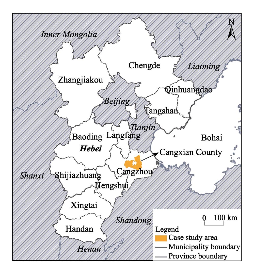
This study is carried out in one of the typical agricultural production counties in the NCP, i.e., Cangxian County, which is located to the south of Beijing and Tianjin and to the east of the Bohai Sea (Fig. 1). Cangxian County has diverse soil types and a temperate monsoon climate. The dominant CS used to be the winter wheat - summer maize double CS, and groundwater is the primary irrigation water source. However, a number of farms have changed to the cultivation of the maize single CS instead of the traditional double CS since the late 1990s (Wang et al., 2016). Since 2014, Cangxian County has become one of the pilot areas for the fallow land policy in the NCP.

Household survey data collected between March and May in 2015 are the main data used in this study. During the household survey process, a stratified random sampling method was applied to choose households within the 35 villages randomly selected in the case study area, and 9-12 households were randomly selected in each village. Semi-structured one-on-one interviews were conducted with the household heads in order to gather the information for agricultural year 2013-2014. Ultimately, we received 350 valid household questionnaires from the 35 villages.

The household questionnaire mainly contains information about the households and their land plots, including the physical information for each land plot, e.g., land quality, plot size, land ownership, and so on. Specific information regarding inputs (labor, seed, machinery, fertilizer, pesticide and irrigation) and outputs (i.e., quantities of wheat and maize) were also gathered. In addition, we recorded the demographic characteristics of the household members, e.g., age, education status, occupation, and income.

The stochastic production frontier approach was selected for quantifying the impacts of LF and CS on farm performance in the case study area. Specifically, the impact on productivity was identified by setting relevant indicators as independent variables in the stochastic production frontier function, while the impact on TE could be identified by setting the potential indicators in the technical inefficiency model.

The stochastic production frontier model regards the grain output as a stochastic production process, using the multiple-input one-output production function as follows:

where X represents a vector of inputs, A represents the technology parameter vector, and f(·) represents the production frontier function. The subscripts i represent individual households. Therefore, Q_i is the output that should be obtained for household i, which is no smaller than the observed output Q₀ of household i due to inefficiency and other factors, i.e., the error term (ε_i). ε_i can be decomposed into two components:

where v_i represents the noise, which is assumed to have a distribution that is identical to and independent from N(0, $\sigma _{v}^{2}$), while μ_i is an unobservable random variable with a non-negative value and represents the inefficiency effect of the observations. The distribution of μ_i is assumed to be N(μ_i, $\sigma _{{{\mu }_{i}}}^{2}$)⁺. The mean μ_i can be defined using the following technical inefficiency model:

where${{W}_{di}}$represents the d-th explanatory variable relevant to the inefficiency of household i, and δ₀ and δ_d represent the coefficients to be estimated.

The isoquant curve of the fully efficient producer (Isoquant curve 1) permits the measurement of TE (Fig. 2). Suppose that LF is one of the inputs for grain producers, then a household operating at point A has achieved full efficiency. However, a household operating at point B suffers from a technical inefficiency effect, whose TE can be expressed as:

where TE ranges between zero and one, and is inversely correlated with the inefficiency effect; OA and OB refer to different levels of production.

The maximum likelihood estimation (MLE) method is usually applied to estimate the parameters, and the likelihood function is constructed using two variance parameters, ${{\sigma }^{2}}=\sigma _{v}^{2}+\sigma _{\mu }^{2}$ and $\gamma =\sigma _{\mu }^{2}/{{\sigma }^{2}}$. Specifically, g represents the ratio of the variance of household-specific TE to the total variance of grain output, which ranges between zero and one. According to Battese and Coelli (1995), if g is not significantly different from zero, then the variance of the inefficiency effects should be zero. In addition, the traditional mean response function should be applicable, in which variables influencing technical inefficiency can be included directly in the production frontier function.

The production frontier function for grain producers in the case study area can be specified using the Cobb-Douglas production function, which is widely applied in many studies relevant to agricultural production in China because of its suitability for Chinese agriculture and lower probability of multicollinearity compared with the translog production function, i.e., an alternative to the Cobb-Douglas production function (Lin, 1992; Qin et al., 2011; Yang et al., 2017). Empirically, the Cobb-Douglas production frontier function for household i is set as:

where Y_i is the grain output (kg ha^-1) of household i during the agricultural year 2013-2014, which is estimated by dividing the total production of wheat and maize by the total agricultural land area of household i. Crops other than wheat and maize are ignored in the models in this study, as the proportion of their combined sown areas to the total area investigated is quite small (less than 3%). The X’s are the production inputs, including labor, seed, machinery, fertilizer, pesticide and irrigation; as indicated by j=1, 2, …, 6. The input costs are obtained separately for wheat and maize grown in a land plot, and they are then added for both crops for each household. As irrigation inputs contain zero values for a number of households, they should be specified as ln{max(Irrigation, 1-Irrigation users)} (Battese and Coelli, 1995). Here, Irrigation users is treated as a dummy variable, as there are zero values of Irrigation. The Z_ik are the variables representing LF and CS, which are included in some of the modeled estimates. Specifically, average plot size (Average_size) is selected as the indicator of LF, as it was often used in previous studies (Rahman and Rahman, 2008; Tan et al., 2010). A smaller value of Average_size implies a weaker connectivity and a more fragmented landscape. The multiple cropping index (MCI) represents the CS and is estimated as the ratio of total areas sown with wheat ($Wheat\_are{{a}_{i}}$) and maize ($Maize\_are{{a}_{i}}$) to the total farmland area (Area_i) of household i.

The value of MCI ranges between one and two (Table 1). It takes the value of one when all land plots adopt the maize single CS and it approaches two when all land plots adopt the wheat-maize double CS. Therefore, a larger MCI_i indicates that more land plots grow wheat in household i. The final variables, v_i and μ_i, have the same meanings as in equation (2).

The empirical technical inefficiency model is set as:

where the M_di are household specific characteristics which explain inefficiency, and are considered to effect productivity indirectly by influencing TE. In this study, average land quality (Qland_i) is considered to be one of the likely indicators influencing TE, which is defined as the ratio of the aggregate product of the land quality (Land_quality_ik) and area (Area_ik) for each land plot to the total farmland area (Area_i) for household i.

There are four grades for Land_quality_ik: 1 for good land, 2 for relatively good land, 3 for relatively poor land and 4 for poor land, as judged mainly by the results obtained during the implementation of the HRS in the study area (Wang and Li, 2018a). Thus, a high Qland value indicates a low LQ, and the lower the Qland, the better the LQ.

Additional indicators in this model include the age and education of the household head, the ratio of agricultural labor to family size (Ragrilabor), the ratio of off-farm labor to total labor (Routlabor) and the average income per off-farm labor (Aincome). The Z’s have the same meanings as in equation (5). ${{\omega }_{i}}$ is the unobservable random error, which has an independent distribution.

In this study, we assume that LF and CS have effects on both farm productivity and efficiency, and therefore, we develop four distinct models with different variables included. In Model 1, only six input variables are considered in the production frontier function, while the indicators representing LF and CS, i.e., Average_size and MCI, and other indicators representing land quality and household characteristics are included in the inefficiency model. In Model 2, the production frontier function includes both the input variables and the Average_size, while the MCI are included in the inefficiency model. In Model 3, we assume that productivity can be influenced by CS, without considering LF. Therefore, the MCI is in the production frontier function, while the Average_size is included in the inefficiency model. In contrast, Model 4 considers the impacts of LF and CS on productivity, and the Average_size and the MCI are both considered in the production frontier function, rather than in the inefficiency model.

The TE of household i (TE_i) can be empirically estimated by obtaining the expressions for the conditional expectation μ_i upon the observed value of ε_i.

(9) $T{{E}_{i}}=\text{E}(\left. \text{exp(}-{{\mu }_{i}}\text{)} \right|{{\varepsilon }_{i}})$

Table 1 presents the descriptions and summary statistics for all of the variables in equation (5) and equation (7).

Table 1 shows that the average plot size of the sample households is 0.16 ha. This is much larger than that in the mountainous areas of Southwest China, such as Chongqing City (0.05 ha), while it equals the average plot size in Jiangsu Province (0.16 ha) and represents only one-fourth of the average plot size for rice production plots in the Jianghan Plain (0.60 ha) (Wang et al., 2017; Lu et al., 2018; Wang et al., 2019). Both the single CS and the double CS are common in the case study area, with the average MCI equal to 1.55. The land quality is not good, as the average value of Qland equals 2.01. Household heads are usually relatively old and have low education levels, because the average values for Age and Education are 56.92 and 2.29, respectively. In addition, family size and non-agricultural income are often regarded as potential factors influencing farmers’ efficiency. The average ratio of agricultural labor to the family size is 0.49, while the average ratio of off-farm labor to total labor is 0.35. For the off-farm laborers, their average income is 1.24×10⁴ yuan person^-1 yr^-1.

As mentioned above, the MLE method is applied to obtain the parameters for the Cobb-Douglas production frontier and technical inefficiency models, and their results confirm that the γ values in the four models are all significantly different from zero (Table 2). Therefore, the μ term should be estimated using an inefficiency model. The estimated coefficients for the same independent variable in the four models usually have consistent signs and the magnitudes of changes are small, implying that the results are robust with respect to parameter specification.

In the next two sections, we will first analyze the results of the production frontier functions, and then turn to the results of the inefficiency models.

The upper part of Table 2 shows the results of the production frontier models. Four of the six basic production input variables (i.e., labor, seed, pesticide and irrigation) significantly influence farmers’ productivity. Labor proves to be the most important of them, as its coefficient is the largest, and the increase in labor input can improve farm productivity. With respect to seed and irrigation, increases in their inputs also contribute to the improvement of grain output, although they have smaller coefficients than labor. In comparison, the coefficients of pesticide are negative and significant in all models, which may be due to the fact that pesticide is used more extensively in land plots that suffer from more diseases and pests, where outputs are lower. Therefore, this variable can be regarded as an inverse proxy for diseases and pests. In terms of machinery and fertilizer, their impacts on farm productivity are not significant, implying that they may be sources of excessive investment without causing obvious improvements in agricultural performance.

The coefficients of the LF variable (i.e., Average_size), are positive and significant in both Model 2 and Model 4, indicating that Average_size is positively related to grain output and the improvement of LF (i.e., larger values of Average_size) can significantly enhance the farm productivity in the case study area. The reason for this effect may be that LF induces the non-productive inputs, including labor, seed, and land, which reduces the output. The same relationship was found for the rice producers in the Jianghan Plain and the grain producers in the mountainous areas of Chongqing City (Wang et al., 2017; Wang et al., 2019). The MCI also showed positive signs in the production functions in Model 3 and Model 4, meaning that a larger MCI is associated with a higher output; and, in contrast, the adoption of the single CS significantly weakens farm productivity. The intensified land use type, represented by the double CS, is conducive to obtaining a high output, mainly due to the efficient utilization of farm inputs.

The household specific scores of TE can be calculated using equation (9), and the corresponding summary statistics are listed in Table 3. Specifically, Model 1, with the LF and CS variables both included in the inefficiency model, gives the lowest average TE score for the households, while Model 4, with the above variables both included in the production frontier models, estimates the largest average TE score. The value of the average TE in Model 2 is 80.2%, implying that the household can increase its productivity by about 24.69% [(100-80.2)´100/80.2], given the current technology status and the level of inputs. In Model 1, the household productivity can be increased by about 35.69% [(100-73.7)´ 100/73.7], which is the highest among the four models. In addition, the household TE takes a value between 33.0% (Model 1) and 96.7% (Model 2), showing a wide range of variation.

The results of the technical inefficiency models are listed in the lower part of Table 2. Considering that technical inefficiency is specified as the dependent variable, a negative parameter coefficient indicates a negative effect of that independent variable on technical inefficiency, and thus, a positive impact on TE.

According to the results of Model 1, the coefficient of Age is positive, meaning that the older the household head is, the less technically efficient the household will be. This can be explained by the fact that the production management capacity and the ability to obtain new technologies of older farmers are not as good as those of younger farmers. This was also found to be the case for the rice-planting farmers in the Jianghan Plain (Wang et al., 2017). The coefficient of Education is not significant, indicating that a high educational level is not necessary for grain production in the case study area. The impacts of some other indicators including Ragrilabor and Aincome are not significant, but the coefficient of Routlabor is positive, implying that households with a larger ratio of off-farm labor to total labor suffer from a lower level of efficiency. This implies that the off-farm employment can dampen the enthusiasm of the farmers to produce and diminish their TE. With respect to land quality, a positive impact on technical inefficiency is noted for the Qland, implying that the households with better land quality (i.e., lower values of Qland) are less likely to suffer from technical inefficiency, and thus, they are more likely to achieve higher TE values. This has also been reported by a previous study of Wang et al. (2017) .

The Average_size is estimated to be significantly and negatively associated with technical inefficiency. In other words, LF shows a detrimental effect on TE, which should be attributed to the additional costs for households caused by LF, including the waste of inputs, the requirement of more travelling time, and consumption of working hours for labor when travelling between the homestead and land plots. This confirms the findings of Rahman and Rahman (2008) and Jia et al. (2017), who found an inverse relationship between the LF and TE for individual crops, such as rice and barley. This is also similar to the findings of Qin et al. (2011) and Manjunatha et al. (2013), who reported that LF is negatively associated with TE when multiple crops are taken into consideration. The coefficient of MCI for technical inefficiency is significant and negative, meaning that adopting the double CS can significantly improve TE and abandoning winter wheat can lead to a decrease of TE. A previous study by Yang et al. (2017) also found that MCI was positively correlated with the TE in the NCP, which is consistent with the finding of this study.

The results of this study show that the farm productivity and efficiency of grain producers are significantly influenced by both the LF and the CS in the case study area. Specifically, LF plays a detrimental role in both farm productivity and efficiency due to its negative management effect. Considering that increases of farm productivity and efficiency are of crucial importance for the food supply in major food production areas like the NCP in China, and fragmented land is usually regarded as a bottleneck, policies aiming to reduce LF are strongly needed. Our results also show that Routlabor is significantly positive for technical inefficiency, implying that the households with large ratios of out-migration labor usually suffer from low values of TE. In this context, land transfers, from the households with large ratios of out-migration labor to those with ample agricultural labor or to agricultural cooperatives, may be a good solution for decreasing LF by aggregating the scattered land plots into large blocks, and can therefore increase farm productivity and efficiency (Feng, 2008; Shao et al., 2015). However, the average ratio of land transfer in the case study area (4%) is much lower than that in China as a whole (35%) (Wang and Li, 2018a). Policies concerning land market improvements and rural land reconfirmations are suggested, with the goal of facilitating access to the land rental market and increasing longer-term land transfers (Feng, 2008; Ding and Zhong, 2017).

We are also concerned about the impact of household CS on productivity and efficiency, and the results show that the influences of the CS variable, i.e., the MCI, are significant in both the production frontier and inefficiency models. Specifically, the MCI values vary among the households in the case study area, and the households adopting larger proportions of double CS, i.e., those with larger values of MCI, usually experience higher levels of farm productivity and efficiency. However, the NCP is suffering from the abandonment of winter wheat due to the fallow land policy, which aims to alleviate the groundwater overexploitation. This inevitably causes a decrease of the MCI and thus plays a detrimental role in the productivity and efficiency of grain producers in the NCP, the bread basket of China, which may ultimately affect the stable supply of grain products in the NCP (Zhong et al., 2017). Previous studies have analyzed the effects of diversified crop rotations on groundwater consumption and food production in the NCP, and they concluded that compared with the traditional double CS and the single CS, diversifying crop rotations, such as triple cropping in two years and quadruple cropping in three years, usually resulted in smaller values for annual average groundwater decline and larger values for water use efficiency (Meng et al., 2012; Yang et al., 2015). Therefore, we suggest that diversifying crop rotations, instead of just the single CS proposed by the central government, may be a better solution for mitigating the groundwater overexploitation while guaranteeing the agricultural productivity, efficiency and food supply in the NCP (Yang et al., 2015; Wang et al., 2016).

Previous case studies were mainly concerned with the impact of LF on productivity and efficiency for a single crop. However, farmers make land use decisions considering the profit of the whole farm, rather than the profit of just a single crop. In this study, we consider the major crops, i.e., wheat and maize, and analyze the impacts of both LF and CS on productivity and efficiency for grain producers in the NCP, using Cangxian County of Hebei Province as an example. The average plot size (Average_size) and the multiple cropping index (MCI) are selected as indicators for representing LF and CS, respectively. The results show that the coefficients of the Average_size and the MCI are both significant and positive in the production frontier functions, but the coefficients of these two indicators are both significant and negative in the technical inefficiency models. Therefore, LF plays significant and detrimental roles in both farm productivity and efficiency; and the wheat-maize double CS, rather than the maize single CS, is usually associated with high farm productivity and efficiency. In addition to LF and CS, farmers’ productivity is also significantly influenced by four basic production input variables, including labor, seed, pesticide and irrigation. The age of the household head and the ratio of off-farm labor to total labor are also found to be significantly relevant in determining TE.

This study has quantified the impacts of LF and CS on the productivity and efficiency of grain producers in Cangxian County of the NCP. Based on the main findings of this study, it has uncovered the potential for achieving the twin goals of water conservation and food security from the perspective of the promotion of land transfer, and the adjustment of the cropping systems in the NCP. These findings are meaningful and applicable in other cases concerning the promotion of the land productivity and TE in areas with fragmented land and water shortage problems, not just in China, but around the world.

References

[1] Battese GE, Coelli TJ. A model for technical inefficiency effects in a stochastic frontier production function for panel data. Empirical Economics, 20, 325-332(1995).
[3] DingL, Zhong ZB. Influences of rural land reconfirmation on rural land circulation: A case study of Hubei Province. Research of Agricultural Modernization, 38, 452-459(2017).
[4] FengS. Land rental, off-farm employment and technical efficiency of farm households in Jiangxi Province, China. NJAS: Wageningen Journal of Life Sciences, 55, 363-378(2008).
[6] JiaX, SunZ, LiX. The technical efficiency and its influencing factors of barley production in China: A case study of a survey data of barley farmers in 12 provinces. Research of Agricultural Modernization, 38, 713-719(2017).
[7] LinY. Rural reforms and agricultural growth in China. The American Economic Review, 82, 34-51(1992).
[9] LuH, XieH, HeY et al. Assessing the impacts of land fragmentation and plot size on yields and costs: A translog production model and cost function approach. Agricultural Systems, 161, 81-88(2018).
[11] McPherson MF. Land fragmentation: A selected literature review. Development Discussion Paper No. 141. Harvard Institute for International Development. Harvard University.(1982).
[12] MengQ, SunQ, ChenX et al. Alternative cropping systems for sustainable water and nitrogen use in the North China Plain. Agriculture, Ecosystems & Environment, 146, 93-102(2012).
[14] QinL, ZhangN, JiangZ. Land fragmentation, labor out-migration and the household agricultural production in China: Findings from surveys in Anhui Province. Journal of Agrotechnical Economics, 16-23(2011).
[18] TanS, HeerinkN, KuyvenhovenA et al. Impact of land fragmentation on rice producers’ technical efficiency in South-East China. NJAS: Wageningen Journal of Life Sciences, 57, 117-123(2010).
[26] WangY, LiX, XinL. Characteristics of cropland fragmentation and its impact on agricultural production costs in mountainous areas. Journal of Natural Resources, 34, 2658-2672(2019).
[29] YangY, DengX, LiZ et al. Impact of land use change on grain production efficiency in North China Plain during 2000-2015. Geographical Research, 36, 2171-2183(2017).
[30] YangZ. To further ascertain peasants’ land use rights. Agricultural Economics Problems, 48-52(1995).
[31] YaoY. The system of farmland in China: An analytical framework. Social Science in China, 54-65(2000).
[36] ZhouS, WangY, ZhuS. The technical efficiency and its influencing factors of peanut production in China: Findings from household survey data in 19 provinces. 3): 27-, 36, 46(2013).
Xue WANG, Xiubin LI. Impacts of Land Fragmentation and Cropping System on the Productivity and Efficiency of Grain Producers in the North China Plain: Taking Cangxian County of Hebei Province as an Example[J]. Journal of Resources and Ecology, 2020, 11(6): 580