
Hao Wan, Lei Lei, Rui Li, Wei Chen, Yiqing Shi. Cloud Detection in Landsat8 OLI Remote Sensing Image with Dual Attention Mechanism[J]. Laser & Optoelectronics Progress, 2023, 60(14): 1428004
- Laser & Optoelectronics Progress
- Vol. 60, Issue 14, 1428004 (2023)
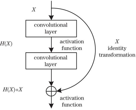
Fig. 1. Structure of ResNet model

Fig. 2. Improved densely connected modules
Fig. 3. Conversion module
Fig. 4. Bottleneck structure. (a) Traditional bottleneck structure; (b) improved bottleneck structure
Fig. 5. Channel attention module
Fig. 6. Location attention module
Fig. 7. NLNet module structure
Fig. 8. Global context modeling module
Fig. 9. Atrous convolution module
Fig. 10. Densely connected network incorporating attention mechanism
Fig. 11. Ratio of image blocks covered by thick and thin clouds in different datasets
Fig. 12. Detection results of thin and thick clouds over land and coastal areas. (a) Original composite image (land); (b) cloud detection results of proposed algorithm (land); (c) original composite image (ocean); (d) cloud detection results of proposed algorithm (ocean)
Fig. 13. Detection results of different cloud detection methods in scenario 1. (a) Original composite image; (b) real image of the ground; (c) F-CNN algorithm; (d) proposed algorithm+no multi-scale; (e) RF algorithm; (f) SVM algorithm; (g) proposed algorithm; (h) Fmask algorithm
Fig. 14. Detection results of different cloud detection methods in scenario 2. (a) Original composite image; (b) real image of the ground; (c) F-CNN algorithm; (d) proposed algorithm+no multi-scale; (e) RF algorithm; (f) SVM algorithm; (g) proposed algorithm; (h) Fmask algorithm
Fig. 15. Detection results of different cloud detection methods in scenario 3. (a) Original composite image; (b) real image of the ground; (c) F-CNN algorithm; (d) proposed algorithm+no multi-scale; (e) RF algorithm; (f) SVM algorithm; (g) proposed algorithm; (h) Fmask algorithm
Fig. 16. Test datasets cloud detection accuracy distribution map. (a) Comparison with F-CNN model; (b) comparison with self-contrast model; (c) comparison with RF model; (d) comparison with SVM model
Fig. 17. RR distribution of cloud test datasets
Fig. 18. ER distribution of cloud test datasets
Fig. 19. FAR distribution of cloud test dataset
Fig. 20. RER distribution of cloud test datasets
|
Table 1. Image distribution of cloud coverage in train and test datasets
|
Table 2. Detection performance of different methods for thick and thin clouds
|
Table 3. Full cloud detection performance of different methods
|
Table 4. Ablation experiment results

Set citation alerts for the article
Please enter your email address
© Copyright 2018-2021 | Chinese Laser Press. All Rights Reserved 沪ICP备15018463号-20